Table of Contents
Data Drift/Shift
- Types of SHIFT:
- Dataset shift happens when the i.i.d. assumptions are not valid for out problem space
- Types of SHIFT:
-
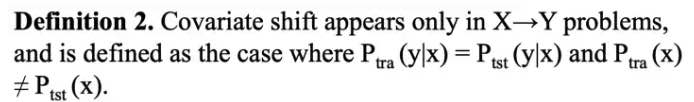
Covariate Shift:
-
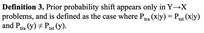
Prior Probability Shift: \(P(x)\)
-
Covariate Shift:
-
Internal CS:
Researchers found that due to the variation in the distribution of activations from the output of a given hidden layer, which are used as the input to a subsequent layer, the network layers can suffer from covariate shift which can impede the training of deep neural networks.-
Covariate shift is the change in the distribution of the covariates specifically, that is, the independent variables. This is normally due to changes in state of latent variables, which could be temporal (even changes to the stationarity of a temporal process), or spatial, or less obvious.
-
IIt introduces BIAS to cross-validation
-
-
The problem of dataset shift can stem from the way input features are utilized, the way training and test sets are selected, data sparsity, shifts in the data distribution due to non-stationary environments, and also from changes in the activation patterns within layers of deep neural networks.
-
- General Data Distribution Shifts:
- Feature change, such as when new features are added, older features are removed, or the set of all possible values of a feature changes: months to years
-
Label schema change is when the set of possible values for Y change. With label shift, P(Y) changes but P(X Y) remains the same. With label schema change, both P(Y) and P(X Y) change. - CREDIT: * With regression tasks, label schema change could happen because of changes in the possible range of label values. Imagine you’re building a model to predict someone’s credit score. Originally, you used a credit score system that ranged from 300 to 850, but you switched to a new system that ranges from 250 to 900.
- Causes of SHIFT:
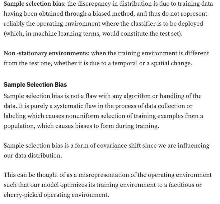
- Dataset shift resulting from sample selection bias is especially relevant when dealing with imbalanced classification, because, in highly imbalanced domains, the minority class is particularly sensitive to singular classification errors, due to the typically low number of samples it presents.
- IN CREDIT
- Non-stationary due to changing macro-economic state
- Adversarial Relationship / Fraud: people might try to game the system to get loans
- Handling Data Distribution Shifts:
- DETECTION
- HANDLING
- DETECTION:
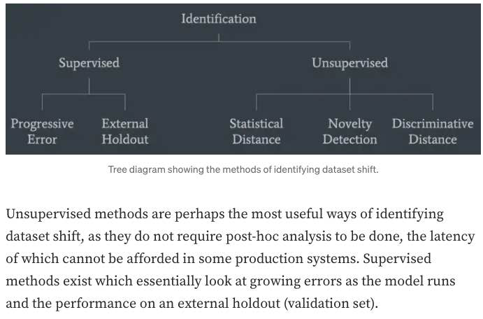
- monitor your model’s accuracy-related metrics30 in production to see whether they have changed.
-
When ground truth labels are unavailable or too delayed to be useful, we can monitor other distributions of interest instead. The distributions of interest are the input distribution P(X), the label distribution P(Y), and the conditional distributions P(X Y) and P(Y X). - In research, there have been efforts to understand and detect label shifts without labels from the target distribution. One such effort is Black Box Shift Estimation by Lipton et al., 2018.
-
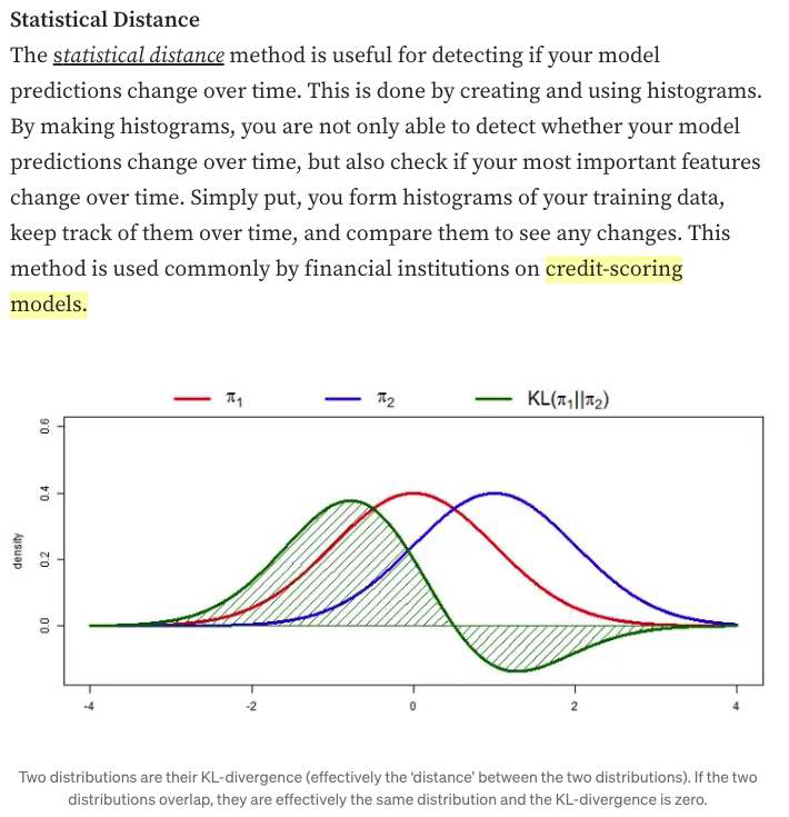
- Statistical Methods:
- a simple method many companies use to detect whether the two distributions are the same is to compare their statistics like mean, median, variance, quantiles, skewness, kurtosis, etc. (bad)
- If those metrics differ significantly, the inference distribution might have shifted from the training distribution. However, if those metrics are similar, there’s no guarantee that there’s no shift.
- a simple method many companies use to detect whether the two distributions are the same is to compare their statistics like mean, median, variance, quantiles, skewness, kurtosis, etc. (bad)
- monitor your model’s accuracy-related metrics30 in production to see whether they have changed.
Encoding
-
Linear Algebra:
-
Linear Algebra:
-
Linear Algebra:
-
Linear Algebra:
Feature Importance
-
Linear Algebra:
-
Linear Algebra:
-
Linear Algebra:
-
Linear Algebra:
Feature Selection
-
Linear Algebra:
-
Linear Algebra:
-
Linear Algebra:
-
Linear Algebra:
Data Preprocessing and Normalization
-
Linear Algebra:
-
Linear Algebra:
Data Regularization:
- The Design Matrix contains sample points in each row
- Feature Scaling/Mean Normalization (of data):
- Define the mean \(\mu_j\) of each feature of the datapoints \(x^{(i)}\):
$$\mu_{j}=\frac{1}{m} \sum_{i=1}^{m} x_{j}^{(i)}$$
- Replace each \(x_j^{(i)}\) with \(x_j - \mu_j\)
- Centering: subtracting \(\mu\) from each row of \(X\)
- Sphering: applying the transform \(X' = X \Sigma^{-1/2}\)
- Whitening: Centering + Sphering (also known as Decorrelating feature space)
Why Normalize the Data/Signal?

-
Linear Algebra:
-
CODE:
Validation & Evaluation - ROC, AUC, Reject Inference + Off-policy Evaluation
-
Linear Algebra:
- ROC:
- A way to quantify how good a binary classifier separates two classes
- True-Positive-Rate / False-Positive-Rate
- Good classifier has a ROC curve that is near the top-left diagonal (hugging it)
- A Bad Classifier has a ROC curve that is close to the diagonal line
- It allows you to set the classification threshold
- You can minimize False-positive rate or maximize the True-Positive Rate
Notes:
- ROC curve is monotone increasing from 0 to 1 and is invariant to any monotone transformation of test results.
- ROC curves (& AUC) are useful even if the predicted probabilities are not “properly calibrated”
- ROC curves are not affected by monotonically increasing functions
- Scale and Threshold Invariance (Blog)
- Accuracy is neither a threshold-invariant metric nor a scale-invariant metric.
-
When to use PRECISION: when data is imbalanced E.G. when the number of negative examples is larger than positive.
Precision does not include TN (True Negatives) so NOT AFFECTED.
In PRACTICE, e.g. studying RARE Disease.
- ROC Curve only cares about the ordering of the scores, not the values.
-
Probability Calibration and ROC: The calibration doesn’t change the order of the scores, it just scales them to make a better match, and the ROC score only cares about the ordering of the scores.
- AUC: The AUC is also the probability that a randomly selected positive example has a higher score than a randomly selected negative example.

-
AUC:
AUC provides an aggregate measure of performance across all possible classification thresholds. One way of interpreting AUC is as the probability that the model ranks a random positive example more highly than a random negative example.-
Range \(= 0.5 - 1.0\), from poor to perfect
- Pros:
- AUC is scale-invariant: It measures how well predictions are ranked, rather than their absolute values.
- AUC is classification-threshold-invariant: It measures the quality of the model’s predictions irrespective of what classification threshold is chosen.
These properties make AUC pretty valuable for evaluating binary classifiers as it provides us with a way to compare them without caring about the classification threshold.
-
Cons
However, both these reasons come with caveats, which may limit the usefulness of AUC in certain use cases:-
Scale invariance is not always desirable. For example, sometimes we really do need well calibrated probability outputs, and AUC won’t tell us about that.
-
Classification-threshold invariance is not always desirable. In cases where there are wide disparities in the cost of false negatives vs. false positives, it may be critical to minimize one type of classification error. For example, when doing email spam detection, you likely want to prioritize minimizing false positives (even if that results in a significant increase of false negatives). AUC isn’t a useful metric for this type of optimization.
-
Notes:
- Partial AUC can be used when only a portion of the entire ROC curve needs to be considered.
-
- Reject Inference and Off-policy Evaluation:
-
Reject inference is a method for performing off-policy evaluation, which is a way to estimate the performance of a policy (a decision-making strategy) based on data generated by a different policy. In reject inference, the idea is to use importance sampling to weight the data in such a way that the samples generated by the behavior policy (the one that generated the data) are down-weighted, while the samples generated by the target policy (the one we want to evaluate) are up-weighted. This allows us to focus on the samples that are most relevant to the policy we are trying to evaluate, which can improve the accuracy of our estimates.
-
Off-policy evaluation is useful in situations where it is not possible or practical to directly evaluate the performance of a policy. For example, in a real-world setting, it may not be possible to directly evaluate a new policy because it could be risky or expensive to implement. In such cases, off-policy evaluation can help us estimate the performance of the policy using data generated by a different, perhaps safer or more easily implemented, policy.
-
-
Validation:
-
Validate a model with given constraints (see above).
Spoke to the recruiter who was super nice and transparent. Scheduled a technical screening afterwards. The question was to validate a model only knowing the true values and predicted values. The interviewer wanted to incorporate the business value of the model. I found this to be interesting and odd as how can the business value validate any model. As we walked through the problem, the interviewer did not care about traditional statistical error measures and techniques in model validation. The interviewer wanted to incorporate the business cases (i.e. total loss in revenue and gains) to validate the model. To me, it felt more business intelligence rather than traditional statistics/machine learning model validation. I am uncertain if data scientists at Affirm are just BI with Python skills.
-
- Evaluation:
- Precision vs Recall Tradeoff:
-
Recall is more important where Overlooked Cases (False Negatives) are more costly than False Alarms (False Positive). The focus in these problems is finding the positive cases.
-
Precision is more important where False Alarms (False Positives) are more costly than Overlooked Cases (False Negatives). The focus in these problems is in weeding out the negative cases.
-
- Precision vs Recall Tradeoff:
Regularization
-
Regularization:
-
Norms:
-
AUC:
-
Linear Algebra:
Interpretability
-
Regularization:
-
Norms:
-
AUC:
-
Linear Algebra:
Decision Trees, Random Forests, XGB, and Gradient Boosting
-
Regularization:
-
Norms:
-
AUC:
-
Boosting:
-
Boosting:
- Boosting: create different hypothesis \(h_i\)s sequentially + make each new hypothesis decorrelated with previous hypothesis.
- Assumes that this will be combined/ensembled
- Ensures that each new model/hypothesis will give a different/independent output
- Boosting: create different hypothesis \(h_i\)s sequentially + make each new hypothesis decorrelated with previous hypothesis.
Uncertainty and Probabilistic Calibration
- Uncertainty:
- Aleatoric vs Epistemic:
Aleatoric uncertainty and epistemic uncertainty are two types of uncertainty that can arise in statistical modeling and machine learning. Aleatoric uncertainty is a type of uncertainty that arises from randomness or inherent noise in the data. It is inherent to the system being studied and cannot be reduced through additional data or better modeling. On the other hand, epistemic uncertainty is a type of uncertainty that arises from incomplete or imperfect knowledge about the system being studied. It can be reduced through additional data or better modeling.
- Aleatoric vs Epistemic:
-
Model Uncertainty, Softmax, and Dropout:
Interpreting Softmax Output Probabilities:
Softmax outputs only measure Aleatoric Uncertainty.
In the same way that in regression, a NN with two outputs, one representing mean and one variance, that parameterise a Gaussian, can capture aleatoric uncertainty, even though the model is deterministic.
Bayesian NNs (dropout included), aim to capture epistemic (aka model) uncertainty.Dropout for Measuring Model (epistemic) Uncertainty:
Dropout can give us principled uncertainty estimates.
Principled in the sense that the uncertainty estimates basically approximate those of our Gaussian process.Theoretical Motivation: dropout neural networks are identical to variational inference in Gaussian processes.
Interpretations of Dropout:- Dropout is just a diagonal noise matrix with the diagonal elements set to either 0 or 1.
- What My Deep Model Doesn’t Know (Blog! - Yarin Gal)
- Calibration in Deep Networks:
- Linear Algebra:
Extra: Bandit, bootstrapping, and prediction interval estimation, Linear Models in Credit
-
Bandit:
-
bootstrapping:
-
prediction interval estimation:
-
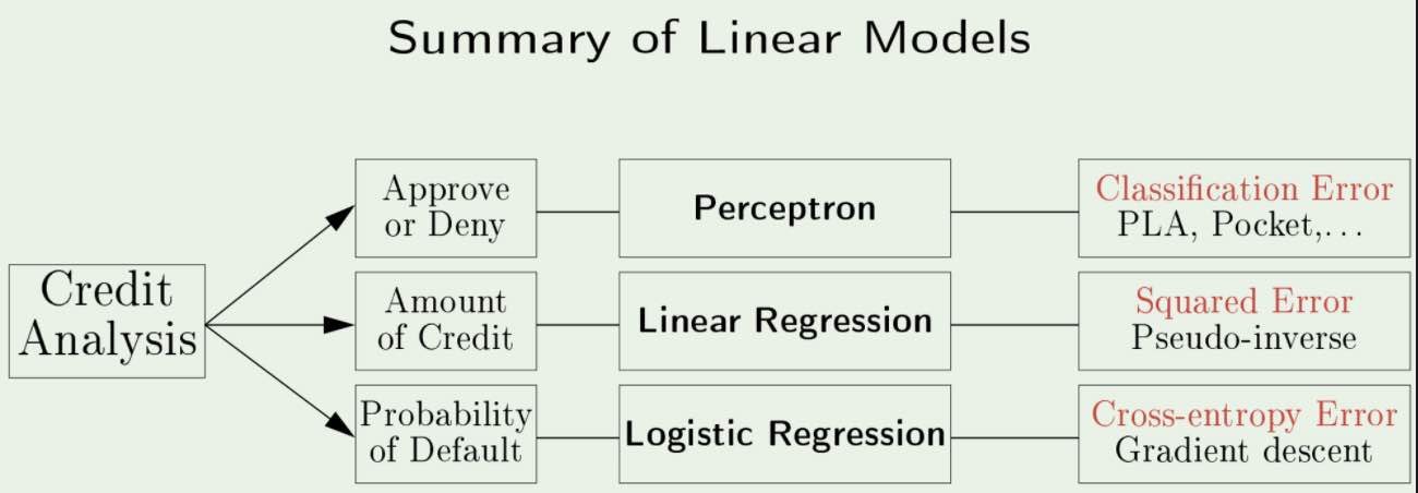
Linear Models in Credit Analysis:
 s
s -
Errors vs Residuals:
The Error of an observed value is the deviation of the observed value from the (unobservable) true value of a quantity of interest.The Residual of an observed value is the difference between the observed value and the estimated value of the quantity of interest.
Notes from Affirm Blog
-
Bandit:
-
bootstrapping:
-
prediction interval estimation:
-
Linear Models in Credit Analysis:
s

Information Theory
-
Information Theory:
Information theory is a branch of applied mathematics that revolves around quantifying how much information is present in a signal.
In the context of machine learning, we can also apply information theory to continuous variables where some of these message length interpretations do not apply, instead, we mostly use a few key ideas from information theory to characterize probability distributions or to quantify similarity between probability distributions.
- Motivation and Intuition:
The basic intuition behind information theory is that learning that an unlikely event has occurred is more informative than learning that a likely event has occurred. A message saying “the sun rose this morning” is so uninformative as to be unnecessary to send, but a message saying “there was a solar eclipse this morning” is very informative.
Thus, information theory quantifies information in a way that formalizes this intuition:- Likely events should have low information content - in the extreme case, guaranteed events have no information at all
- Less likely events should have higher information content
- Independent events should have additive information. For example, finding out that a tossed coin has come up as heads twice should convey twice as much information as finding out that a tossed coin has come up as heads once.
-
Measuring Information:
In Shannons Theory, to transmit \(1\) bit of information means to divide the recipients Uncertainty by a factor of \(2\).Thus, the amount of information transmitted is the logarithm (base \(2\)) of the uncertainty reduction factor.
The uncertainty reduction factor is just the inverse of the probability of the event being communicated.
Thus, the amount of information in an event \(\mathbf{x} = x\), called the Self-Information is:
$$I(x) = \log (1/p(x)) = -\log(p(x))$$
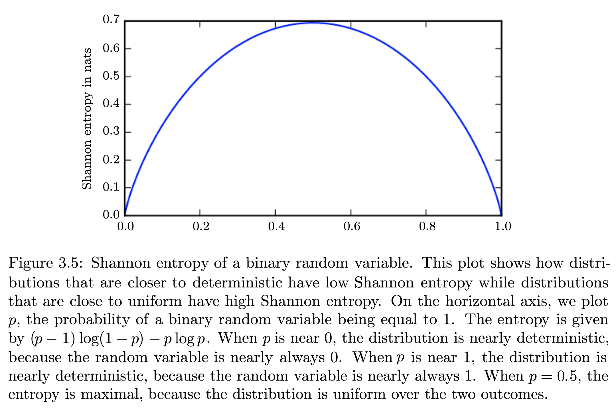
Shannons Entropy:
It is the expected amount of information of an uncertain/stochastic source. It acts as a measure of the amount of uncertainty of the events.
Equivalently, the amount of information that you get from one sample drawn from a given probability distribution \(p\).
- Self-Information:
The Self-Information or surprisal is a synonym for the surprise when a random variable is sampled.
The Self-Information of an event \(\mathrm{x} = x\):$$I(x) = - \log P(x)$$
Self-information deals only with a single outcome.

- Shannon Entropy:
To quantify the amount of uncertainty in an entire probability distribution, we use Shannon Entropy.
Shannon Entropy is defined as the average amount of information produced by a stochastic source of data.$$H(x) = {\displaystyle \operatorname {E}_{x \sim P} [I(x)]} = - {\displaystyle \operatorname {E}_{x \sim P} [\log P(X)] = -\sum_{i=1}^{n} p\left(x_{i}\right) \log p\left(x_{i}\right)}$$
Differential Entropy is Shannons entropy of a continuous random variable \(x\).
-
Distributions and Entropy:
Distributions that are nearly deterministic (where the outcome is nearly certain) have low entropy; distributions that are closer to uniform have high entropy. - Relative Entropy | KL-Divergence:
The Kullback–Leibler divergence (Relative Entropy) is a measure of how one probability distribution diverges from a second, expected probability distribution.
Mathematically:$${\displaystyle D_{\text{KL}}(P\parallel Q)=\operatorname{E}_{x \sim P} \left[\log \dfrac{P(x)}{Q(x)}\right]=\operatorname{E}_{x \sim P} \left[\log P(x) - \log Q(x)\right]}$$
- Discrete:
$${\displaystyle D_{\text{KL}}(P\parallel Q)=\sum_{i}P(i)\log \left({\frac {P(i)}{Q(i)}}\right)}$$
- Continuous:
$${\displaystyle D_{\text{KL}}(P\parallel Q)=\int_{-\infty }^{\infty }p(x)\log \left({\frac {p(x)}{q(x)}}\right)\,dx,}$$
Interpretation:
- Discrete variables:
it is the extra amount of information needed to send a message containing symbols drawn from probability distribution \(P\), when we use a code that was designed to minimize the length of messages drawn from probability distribution \(Q\). - Continuous variables:
Properties:
- Non-Negativity:
\({\displaystyle D_{\mathrm {KL} }(P\|Q) \geq 0}\) - \({\displaystyle D_{\mathrm {KL} }(P\|Q) = 0 \iff}\) \(P\) and \(Q\) are:
- Discrete Variables:
the same distribution - Continuous Variables:
equal “almost everywhere”
- Discrete Variables:
- Additivity of Independent Distributions:
\({\displaystyle D_{\text{KL}}(P\parallel Q)=D_{\text{KL}}(P_{1}\parallel Q_{1})+D_{\text{KL}}(P_{2}\parallel Q_{2}).}\) - \({\displaystyle D_{\mathrm {KL} }(P\|Q) \neq D_{\mathrm {KL} }(Q\|P)}\)
This asymmetry means that there are important consequences to the choice of the ordering
- Convexity in the pair of PMFs \((p, q)\) (i.e. \({\displaystyle (p_{1},q_{1})}\) and \({\displaystyle (p_{2},q_{2})}\) are two pairs of PMFs):
\({\displaystyle D_{\text{KL}}(\lambda p_{1}+(1-\lambda )p_{2}\parallel \lambda q_{1}+(1-\lambda )q_{2})\leq \lambda D_{\text{KL}}(p_{1}\parallel q_{1})+(1-\lambda )D_{\text{KL}}(p_{2}\parallel q_{2}){\text{ for }}0\leq \lambda \leq 1.}\)
KL-Div as a Distance:
Because the KL divergence is non-negative and measures the difference between two distributions, it is often conceptualized as measuring some sort of distance between these distributions.
However, it is not a true distance measure because it is not symmetric.KL-div is, however, a Quasi-Metric, since it satisfies all the properties of a distance-metric except symmetry
Applications
Characterizing:- Relative (Shannon) entropy in information systems
- Randomness in continuous time-series
- It is a measure of Information Gain; used when comparing statistical models of inference
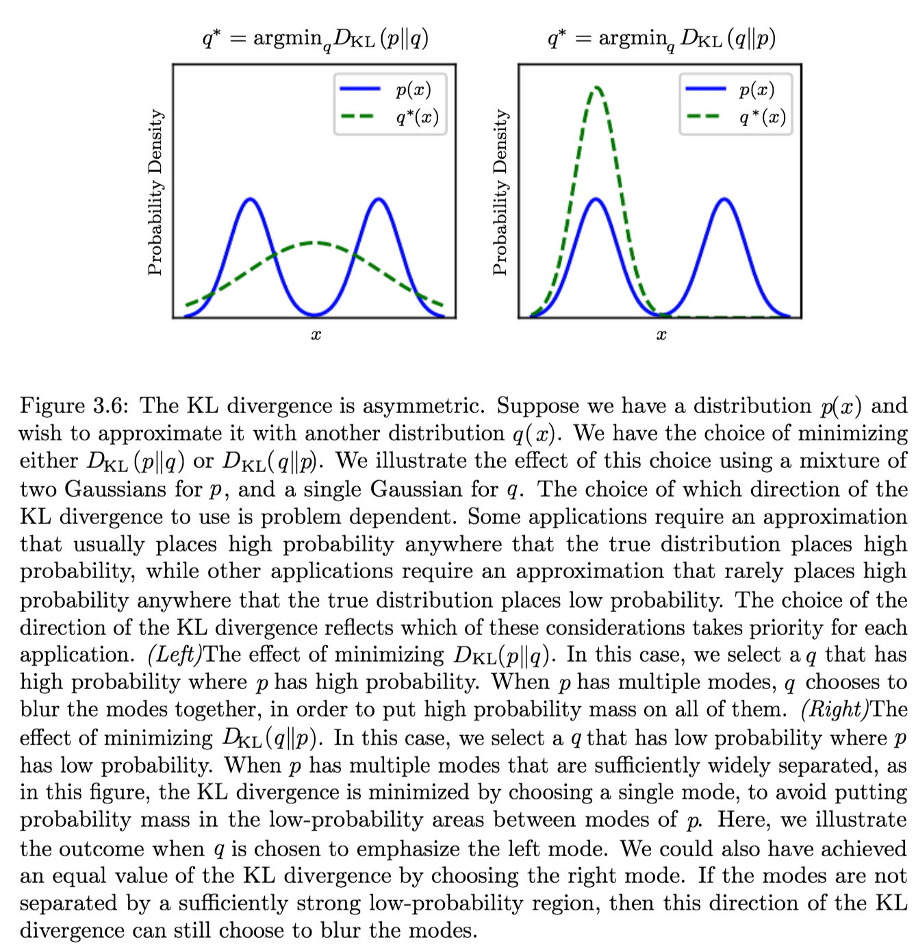
Example Application and Direction of Minimization
Suppose we have a distribution \(p(x)\) and we wish to approximate it with another distribution \(q(x)\).
We have a choice of minimizing either:- \({\displaystyle D_{\text{KL}}(p\|q)} \implies q^\ast = \operatorname {arg\,min}_q {\displaystyle D_{\text{KL}}(p\|q)}\)
Produces an approximation that usually places high probability anywhere that the true distribution places high probability. - \({\displaystyle D_{\text{KL}}(q\|p)} \implies q^\ast \operatorname {arg\,min}_q {\displaystyle D_{\text{KL}}(q\|p)}\)
Produces an approximation that rarely places high probability anywhere that the true distribution places low probability.which are different due to the asymmetry of the KL-divergence
- Cross Entropy:
The Cross Entropy between two probability distributions \({\displaystyle p}\) and \({\displaystyle q}\) over the same underlying set of events measures the average number of bits needed to identify an event drawn from the set, if a coding scheme is used that is optimized for an “unnatural” probability distribution \({\displaystyle q}\), rather than the “true” distribution \({\displaystyle p}\).$$H(p,q) = \operatorname{E}_{p}[-\log q]= H(p) + D_{\mathrm{KL}}(p\|q) =-\sum_{x }p(x)\,\log q(x)$$
It is similar to KL-Div but with an additional quantity - the entropy of \(p\).
Minimizing the cross-entropy with respect to \(Q\) is equivalent to minimizing the KL divergence, because \(Q\) does not participate in the omitted term.
We treat \(0 \log (0)\) as \(\lim_{x \to 0} x \log (x) = 0\).
-
Mutual Information:
The Mutual Information (MI) of two random variables is a measure of the mutual dependence between the two variables.
More specifically, it quantifies the “amount of information” (in bits) obtained about one random variable through observing the other random variable.It can be seen as a way of measuring the reduction in uncertainty (information content) of measuring a part of the system after observing the outcome of another parts of the system; given two R.Vs, knowing the value of one of the R.Vs in the system gives a corresponding reduction in (the uncertainty (information content) of) measuring the other one.
As KL-Divergence:
Let \((X, Y)\) be a pair of random variables with values over the space \(\mathcal{X} \times \mathcal{Y}\) . If their joint distribution is \(P_{(X, Y)}\) and the marginal distributions are \(P_{X}\) and \(P_{Y},\) the mutual information is defined as:$$I(X ; Y)=D_{\mathrm{KL}}\left(P_{(X, Y)} \| P_{X} \otimes P_{Y}\right)$$
In terms of PMFs for discrete distributions:
The mutual information of two jointly discrete random variables \(X\) and \(Y\) is calculated as a double sum:$$\mathrm{I}(X ; Y)=\sum_{y \in \mathcal{Y}} \sum_{x \in \mathcal{X}} p_{(X, Y)}(x, y) \log \left(\frac{p_{(X, Y)}(x, y)}{p_{X}(x) p_{Y}(y)}\right)$$
where \({\displaystyle p_{(X,Y)}}\) is the joint probability mass function of \({\displaystyle X}\) X and \({\displaystyle Y}\), and \({\displaystyle p_{X}}\) and \({\displaystyle p_{Y}}\) are the marginal probability mass functions of \({\displaystyle X}\) and \({\displaystyle Y}\) respectively.
In terms of PDFs for continuous distributions:
In the case of jointly continuous random variables, the double sum is replaced by a double integral:$$\mathrm{I}(X ; Y)=\int_{\mathcal{Y}} \int_{\mathcal{X}} p_{(X, Y)}(x, y) \log \left(\frac{p_{(X, Y)}(x, y)}{p_{X}(x) p_{Y}(y)}\right) d x d y$$
where \(p_{(X, Y)}\) is now the joint probability density function of \(X\) and \(Y\) and \(p_{X}\) and \(p_{Y}\) are the marginal probability density functions of \(X\) and \(Y\) respectively.
Intuitive Definitions:
- Measures the information that \(X\) and \(Y\) share:
It measures how much knowing one of these variables reduces uncertainty about the other.- \(X, Y\) Independent \(\implies I(X; Y) = 0\): their MI is zero
- \(X\) deterministic function of \(Y\) and vice versa \(\implies I(X; Y) = H(X) = H(Y)\) their MI is equal to entropy of each variable
- It’s a Measure of the inherent dependence expressed in the joint distribution of \(X\) and \(Y\) relative to the joint distribution of \(X\) and \(Y\) under the assumption of independence.
i.e. The price for encoding \({\displaystyle (X,Y)}\) as a pair of independent random variables, when in reality they are not.
Properties:
- The KL-divergence shows that \(I(X; Y)\) is equal to zero precisely when the joint distribution conicides with the product of the marginals i.e. when \(X\) and \(Y\) are independent.
- The MI is non-negative: \(I(X; Y) \geq 0\)
- It is a measure of the price for encoding \({\displaystyle (X,Y)}\) as a pair of independent random variables, when in reality they are not.
- It is symmetric: \(I(X; Y) = I(Y; X)\)
- Related to conditional and joint entropies:
$${\displaystyle {\begin{aligned}\operatorname {I} (X;Y)&{}\equiv \mathrm {H} (X)-\mathrm {H} (X|Y)\\&{}\equiv \mathrm {H} (Y)-\mathrm {H} (Y|X)\\&{}\equiv \mathrm {H} (X)+\mathrm {H} (Y)-\mathrm {H} (X,Y)\\&{}\equiv \mathrm {H} (X,Y)-\mathrm {H} (X|Y)-\mathrm {H} (Y|X)\end{aligned}}}$$
where \(\mathrm{H}(X)\) and \(\mathrm{H}(Y)\) are the marginal entropies, \(\mathrm{H}(X | Y)\) and \(\mathrm{H}(Y | X)\) are the conditional entopries, and \(\mathrm{H}(X, Y)\) is the joint entropy of \(X\) and \(Y\).
- Note the analogy to the union, difference, and intersection of two sets:

- Note the analogy to the union, difference, and intersection of two sets:
- Related to KL-div of conditional distribution:
$$\mathrm{I}(X ; Y)=\mathbb{E}_{Y}\left[D_{\mathrm{KL}}\left(p_{X | Y} \| p_{X}\right)\right]$$
- MI (tutorial #1)
- MI (tutorial #2)
Applications:
- In search engine technology, mutual information between phrases and contexts is used as a feature for k-means clustering to discover semantic clusters (concepts)
- Discriminative training procedures for hidden Markov models have been proposed based on the maximum mutual information (MMI) criterion.
- Mutual information has been used as a criterion for feature selection and feature transformations in machine learning. It can be used to characterize both the relevance and redundancy of variables, such as the minimum redundancy feature selection.
- Mutual information is used in determining the similarity of two different clusterings of a dataset. As such, it provides some advantages over the traditional Rand index.
- Mutual information of words is often used as a significance function for the computation of collocations in corpus linguistics.
- Detection of phase synchronization in time series analysis
- The mutual information is used to learn the structure of Bayesian networks/dynamic Bayesian networks, which is thought to explain the causal relationship between random variables
- Popular cost function in decision tree learning.
- In the infomax method for neural-net and other machine learning, including the infomax-based Independent component analysis algorithm
Independence assumptions and low-rank matrix approximation (alternative definition):

As a Metric (relation to Jaccard distance):

- Measures the information that \(X\) and \(Y\) share:
- Pointwise Mutual Information (PMI):
The PMI of a pair of outcomes \(x\) and \(y\) belonging to discrete random variables \(X\) and \(Y\) quantifies the discrepancy between the probability of their coincidence given their joint distribution and their individual distributions, assuming independence. Mathematically:$$\operatorname{pmi}(x ; y) \equiv \log \frac{p(x, y)}{p(x) p(y)}=\log \frac{p(x | y)}{p(x)}=\log \frac{p(y | x)}{p(y)}$$
In contrast to mutual information (MI) which builds upon PMI, it refers to single events, whereas MI refers to the average of all possible events.
The mutual information (MI) of the random variables \(X\) and \(Y\) is the expected value of the PMI (over all possible outcomes).
More
- Conditional Entropy: \(H(X \mid Y)=H(X)-I(X, Y)\)
- Independence: \(I(X, Y)=0\)
- Independence Relations: \(H(X \mid Y)=H(X)\)
DATA PROCESSING
- Non-Negative Matrix Factorization NMF Tutorial
- UMAP: Uniform Manifold Approximation and Projection for Dimension Reduction [better than t-sne?] (Library Code!)
Dimensionality Reduction
Dimensionality Reduction
Dimensionality Reduction is the process of reducing the number of random variables under consideration by obtaining a set of principal variables. It can be divided into feature selection and feature extraction.
Dimensionality Reduction Methods:
- PCA
- Heatmaps
- t-SNE
- Multi-Dimensional Scaling (MDS)
t-SNE | T-distributed Stochastic Neighbor Embeddings
Understanding t-SNE Part 1: SNE algorithm and its drawbacks
Understanding t-SNE Part 2: t-SNE improvements over SNE
t-SNE (statwiki)
t-SNE tutorial (video)
series (deleteme)
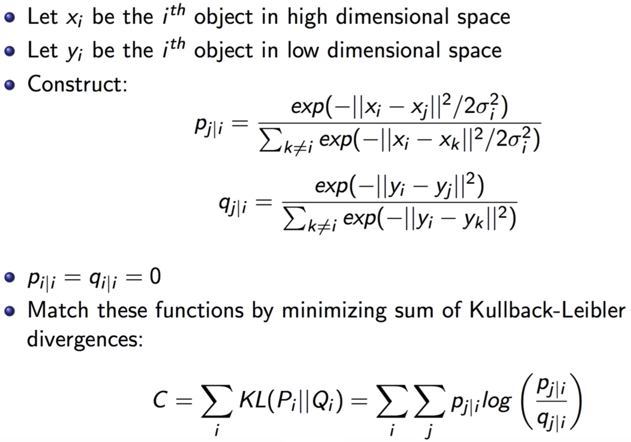
SNE - Stochastic Neighbor Embeddings:
SNE is a method that aims to match distributions of distances between points in high and low dimensional space via conditional probabilities.
It Assumes distances in both high and low dimensional space are Gaussian-distributed.
t-SNE:
t-SNE is a machine learning algorithm for visualization developed by Laurens van der Maaten and Geoffrey Hinton.
It is a nonlinear dimensionality reduction technique well-suited for embedding high-dimensional data for visualization in a low-dimensional space of two or three dimensions.
Specifically, it models each high-dimensional object by a two- or three-dimensional point in such a way that similar objects are modeled by nearby points and dissimilar objects are modeled by distant points with high probability.
It tends to preserve local structure, while at the same time, preserving the global structure as much as possible.
Stages:
- It Constructs a probability distribution over pairs of high-dimensional objects in such a way that similar objects have a high probability of being picked while dissimilar points have an extremely small probability of being picked.
- It Defines a similar probability distribution over the points in the low-dimensional map, and it minimizes the Kullback–Leibler divergence between the two distributions with respect to the locations of the points in the map.
Key Ideas:
It solves two big problems that SNE faces:
- The Crowding Problem:
The “crowding problem” that are addressed in the paper is defined as: “the area of the two-dimensional map that is available to accommodate moderately distant datapoints will not be nearly large enough compared with the area available to accommodate nearby datepoints”. This happens when the datapoints are distributed in a region on a high-dimensional manifold around i, and we try to model the pairwise distances from i to the datapoints in a two-dimensional map. For example, it is possible to have 11 datapoints that are mutually equidistant in a ten-dimensional manifold but it is not possible to model this faithfully in a two-dimensional map. Therefore, if the small distances can be modeled accurately in a map, most of the moderately distant datapoints will be too far away in the two-dimensional map. In SNE, this will result in very small attractive force from datapoint i to these too-distant map points. The very large number of such forces collapses together the points in the center of the map and prevents gaps from forming between the natural clusters. This phenomena, crowding problem, is not specific to SNE and can be observed in other local techniques such as Sammon mapping as well.- Solution - Student t-distribution for \(q\):
Student t-distribution is used to compute the similarities between data points in the low dimensional space \(q\).
- Solution - Student t-distribution for \(q\):
- Optimization Difficulty of KL-div:
The KL Divergence is used over the conditional probability to calculate the error in the low-dimensional representation. So, the algorithm will be trying to minimize this loss and will calculate its gradient:$$\frac{\delta C}{\delta y_{i}}=2 \sum_{j}\left(p_{j | i}-q_{j | i}+p_{i | j}-q_{i | j}\right)\left(y_{i}-y_{j}\right)$$
This gradient involves all the probabilities for point \(i\) and \(j\). But, these probabilities were composed of the exponentials. The problem is that: We have all these exponentials in our gradient, which can explode (or display other unusual behavior) very quickly and hence the algorithm will take a long time to converge.
- Solution - Symmetric SNE:
The Cost Function is a symmetrized version of that in SNE. i.e. \(p_{i\vert j} = p_{j\vert i}\) and \(q_{i\vert j} = q_{j\vert i}\).
- Solution - Symmetric SNE:
Application:
It is often used to visualize high-level representations learned by an artificial neural network.
Motivation:
There are a lot of problems with traditional dimensionality reduction techniques that employ feature projection; e.g. PCA. These techniques attempt to preserve the global structure, and in that process they lose the local structure. Mainly, projecting the data on one axis or another, may (most likely) not preserve the neighborhood structure of the data; e.g. the clusters in the data:
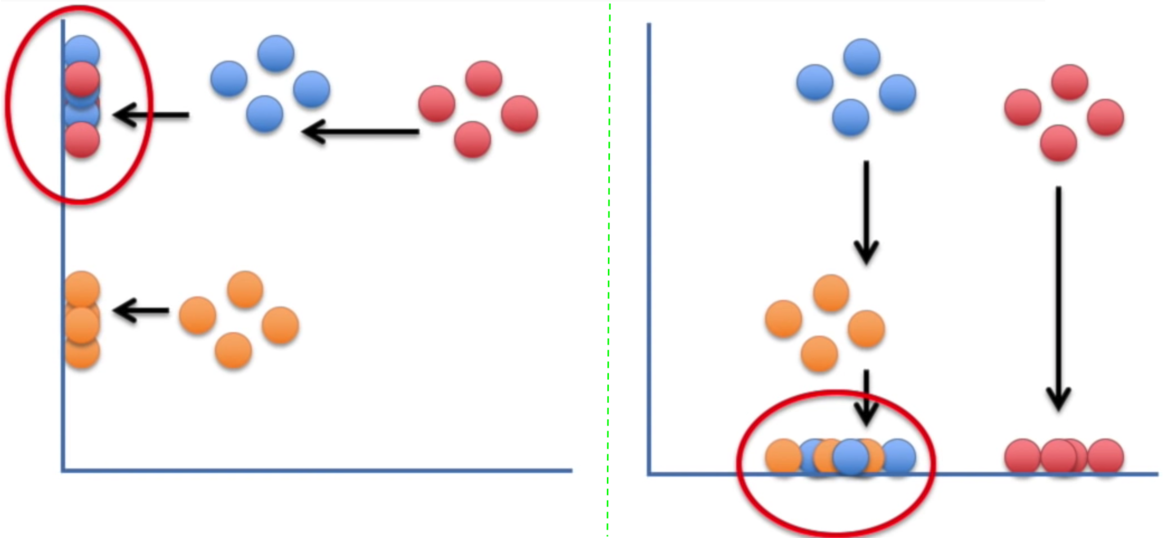
t-SNE finds a way to project data into a low dimensional space (1-d, in this case) such that the clustering (“local structure”) in the high dimensional space is preserved.
t-SNE Clusters:
While t-SNE plots often seem to display clusters, the visual clusters can be influenced strongly by the chosen parameterization and therefore a good understanding of the parameters for t-SNE is necessary. Such “clusters” can be shown to even appear in non-clustered data, and thus may be false findings.
It has been demonstrated that t-SNE is often able to recover well-separated clusters, and with special parameter choices, approximates a simple form of spectral clustering.
Properties:
- It preserves the neighborhood structure of the data
- Does NOT preserve distances nor density
- Only to some extent preserves nearest-neighbors?
discussion - It learns a non-parametric mapping, which means that it does NOT learn an explicit function that maps data from the input space to the map
Algorithm:
Issues/Weaknesses/Drawbacks:
- The paper only focuses on the date visualization using t-SNE, that is, embedding high-dimensional date into a two- or three-dimensional space. However, this behavior of t-SNE presented in the paper cannot readily be extrapolated to \(d>3\) dimensions due to the heavy tails of the Student t-distribution.
- It might be less successful when applied to data sets with a high intrinsic dimensionality. This is a result of the local linearity assumption on the manifold that t-SNE makes by employing Euclidean distance to present the similarity between the datapoints.
- The cost function is not convex. This leads to the problem that several optimization parameters (hyperparameters) need to be chosen (and tuned) and the constructed solutions depending on these parameters may be different each time t-SNE is run from an initial random configuration of the map points.
- It cannot work “online”. Since it learns a non-parametric mapping, which means that it does not learn an explicit function that maps data from the input space to the map. Therefore, it is not possible to embed test points in an existing map. You have to re-run t-SNE on the full dataset.
A potential approach to deal with this would be to train a multivariate regressor to predict the map location from the input data.
Alternatively, you could also make such a regressor minimize the t-SNE loss directly (parametric t-SNE).
t-SNE Optimization:
Discussion and Information:
- What is perplexity?
Perplexity is a measure for information that is defined as 2 to the power of the Shannon entropy. The perplexity of a fair die with k sides is equal to k. In t-SNE, the perplexity may be viewed as a knob that sets the number of effective nearest neighbors. It is comparable with the number of nearest neighbors k that is employed in many manifold learners. - Choosing the perplexity hp:
The performance of t-SNE is fairly robust under different settings of the perplexity. The most appropriate value depends on the density of your data. Loosely speaking, one could say that a larger / denser dataset requires a larger perplexity. Typical values for the perplexity range between \(5\) and \(50\). - Every time I run t-SNE, I get a (slightly) different result?
In contrast to, e.g., PCA, t-SNE has a non-convex objective function. The objective function is minimized using a gradient descent optimization that is initiated randomly. As a result, it is possible that different runs give you different solutions. Notice that it is perfectly fine to run t-SNE a number of times (with the same data and parameters), and to select the visualization with the lowest value of the objective function as your final visualization. - Assessing the “Quality of Embeddings/visualizations”:
Preferably, just look at them! Notice that t-SNE does not retain distances but probabilities, so measuring some error between the Euclidean distances in high-D and low-D is useless. However, if you use the same data and perplexity, you can compare the Kullback-Leibler divergences that t-SNE reports. It is perfectly fine to run t-SNE ten times, and select the solution with the lowest KL divergence.
Feature Selection
Feature Selection
Feature Selection is the process of selecting a subset of relevant features (variables, predictors) for use in model construction.
Applications:
- Simplification of models to make them easier to interpret by researchers/users
- Shorter training time
- A way to handle curse of dimensionality
- Reduction of Variance \(\rightarrow\) Reduce Overfitting \(\rightarrow\) Enhanced Generalization
Strategies/Approaches:
- Wrapper Strategy:
Wrapper methods use a predictive model to score feature subsets. Each new subset is used to train a model, which is tested on a hold-out set. Counting the number of mistakes made on that hold-out set (the error rate of the model) gives the score for that subset. As wrapper methods train a new model for each subset, they are very computationally intensive, but usually provide the best performing feature set for that particular type of model.
e.g. Search Guided by Accuracy, Stepwise Selection - Filter Strategy:
Filter methods use a proxy measure instead of the error rate to score a feature subset. This measure is chosen to be fast to compute, while still capturing the usefulness of the feature set.
Filter methods produce a feature set which is not tuned to a specific model, usually giving lower prediction performance than a wrapper, but are more general and more useful for exposing the relationships between features.
e.g. Information Gain, pointwise-mutual/mutual information, Pearson Correlation - Embedded Strategy:
Embedded methods are a catch-all group of techniques which perform feature selection as part of the model construction process.
e.g. LASSO
Correlation Feature Selection
The Correlation Feature Selection (CFS) measure evaluates subsets of features on the basis of the following hypothesis:
“Good feature subsets contain features highly correlated with the classification, yet uncorrelated to each other”.
The following equation gives the merit of a feature subset \(S\) consisting of \(k\) features:
$${\displaystyle \mathrm {Merit} _{S_{k}}={\frac {k{\overline {r_{cf}}}}{\sqrt {k+k(k-1){\overline {r_{ff}}}}}}.}$$
where, \({\displaystyle {\overline {r_{cf}}}}\) is the average value of all feature-classification correlations, and \({\displaystyle {\overline {r_{ff}}}}\) is the average value of all feature-feature correlations.
The CFS criterion is defined as follows:
$$\mathrm {CFS} =\max _{S_{k}}\left[{\frac {r_{cf_{1}}+r_{cf_{2}}+\cdots +r_{cf_{k}}}{\sqrt {k+2(r_{f_{1}f_{2}}+\cdots +r_{f_{i}f_{j}}+\cdots +r_{f_{k}f_{1}})}}}\right]$$
Feature Selection Embedded in Learning Algorithms
- \(l_{1}\)-regularization techniques, such as sparse regression, LASSO, and \({\displaystyle l_{1}}\)-SVM
- Regularized trees, e.g. regularized random forest implemented in the RRF package
- Decision tree
- Memetic algorithm
- Random multinomial logit (RMNL)
- Auto-encoding networks with a bottleneck-layer
- Submodular feature selection
Information Theory Based Feature Selection Mechanisms
There are different Feature Selection mechanisms around that utilize mutual information for scoring the different features.
They all usually use the same algorithm:
- Calculate the mutual information as score for between all features (\({\displaystyle f_{i}\in F}\)) and the target class (\(c\))
- Select the feature with the largest score (e.g. \({\displaystyle argmax_{f_{i}\in F}(I(f_{i},c))}\)) and add it to the set of selected features (\(S\))
- Calculate the score which might be derived form the mutual information
- Select the feature with the largest score and add it to the set of select features (e.g. \({\displaystyle {\arg \max }_{f_{i}\in F}(I_{derived}(f_{i},c))}\))
- Repeat 3. and 4. until a certain number of features is selected (e.g. \({\displaystyle \vert S\vert =l}\))
Feature Extraction
Feature Extraction
Feature Extraction starts from an initial set of measured data and builds derived values (features) intended to be informative and non-redundant, facilitating the subsequent learning and generalization steps, and in some cases leading to better human interpretations.
In dimensionality reduction, feature extraction is also called Feature Projection, which is a method that transforms the data in the high-dimensional space to a space of fewer dimensions. The data transformation may be linear, as in principal component analysis (PCA), but many nonlinear dimensionality reduction techniques also exist.
Methods/Algorithms:
- Independent component analysis
- Isomap
- Kernel PCA
- Latent semantic analysis
- Partial least squares
- Principal component analysis
- Autoencoder
- Linear Discriminant Analysis (LDA)
- Non-negative matrix factorization (NMF)
Data Imputation
Resources:
Outliers
Replacing Outliers
Data Transformation - Outliers - Standardization
PreProcessing in DL - Data Normalization
Imputation and Feature Scaling
Missing Data - Imputation
Dim-Red - Random Projections
F-Selection - Relief
Box-Cox Transf - outliers
ANCOVA
Feature Selection Methods
PRactiical Concepts
-
Data Snooping:
The Principle:
If a data set has affected any step in the learning process, its ability to assess the outcome has been compromised.Analysis:
- Making decision by examining the dataset makes you a part of the learning algorithm.
However, you didn’t consider your contribution to the learning algorithm when making e.g. VC-Analysis for Generalization. - Thus, you are vulnerable to designing the model (or choices of learning) according to the idiosyncrasies of the dataset.
- The real problem is that you are not “charging” for the decision you made by examining the dataset.
What’s allowed?
- You are allowed (even encouraged) to look at all other information related to the target function and input space.
e.g. number/range/dimension/scale/etc. of the inputs, correlations, properties (monotonicity), etc. - EXCEPT, for the specific realization of the training dataset.
Manifestations of Data Snooping with Examples (one/manifestation):
- Changing the Parameters of the model (Tricky):
- Complexity:
Decreasing the order of the fitting polynomial by observing geometric properties of the training set.
- Complexity:
- Using statistics of the Entire Dataset (Tricky):
- Normalization:
Normalizing the data with the mean and variance of the entire dataset (training+testing).- E.g. In Financial Forecasting; the average affects the outcome by exposing the trend.
- Normalization:
- Reuse of a Dataset:
If you keep Trying one model after the other on the same data set, you will eventually ‘succeed’.
“If you torture the data long enough, it will confess”.
This bad because the final model you selected, is the union of all previous models: since some of those models were rejected by you (a learning algorithm).- Fixed (deterministic) training set for Model Selection:
Selecting a model by trying many models on the same fixed (deterministic) Training dataset.
- Fixed (deterministic) training set for Model Selection:
- Bias via Snooping:
By looking at the data in the future when you are not allowed to have the data (it wouldn’t have been possible); you are creating sampling bias caused by “snooping”.- E.g. Testing a Trading algorithm using the currently traded companies (in S&P500).
You shouldn’t have been able to know which companies are being currently traded (future).
- E.g. Testing a Trading algorithm using the currently traded companies (in S&P500).
Remedies/Solutions to Data Snooping:
- Avoid Data Snooping:
A strict discipline (very hard). - Account for Data Snooping:
By quantifying “How much data contamination”.
- Making decision by examining the dataset makes you a part of the learning algorithm.
-
Mismatched Data:
-
Mismatched Classes:
-
Sampling Bias:
Sampling Bias occurs when: \(\exists\) Region with zero-probability \(P=0\) in training, but with positive-probability \(P>0\) in testing.The Principle:
If the data is sampled in a biased way, learning will produce a similarly biased outcome.Example: 1948 Presidential Elections
- Newspaper conducted a Telephone poll between: Jackson and Truman
- Jackson won the poll decisively.
- The result was NOT unlucky:
No matter how many times the poll was re-conducted, and no matter how many times the sample sized is increased; the outcome will be fixed. - The reason is the Telephone:
(1) Telephones were expensive and only rich people had Telephones.
(2) Rich people favored Jackson.
Thus, the result was well reflective of the (mini) population being sampled.
How to sample:
Sample in a way that matches the distributions of train and test samples.The solution Fails (doesn’t work) if:
\(\exists\) Region with zero-probability \(P=0\) in training, but with positive-probability \(P>0\) in testing.This is when sampling bias exists.
Notes:
- Medical sources sometimes refer to sampling bias as ascertainment bias.
- Sampling bias could be viewed as a subtype of selection bias.
-
Model Uncertainty:
Interpreting Softmax Output Probabilities:
Softmax outputs only measure Aleatoric Uncertainty.
In the same way that in regression, a NN with two outputs, one representing mean and one variance, that parameterise a Gaussian, can capture aleatoric uncertainty, even though the model is deterministic.
Bayesian NNs (dropout included), aim to capture epistemic (aka model) uncertainty.Dropout for Measuring Model (epistemic) Uncertainty:
Dropout can give us principled uncertainty estimates.
Principled in the sense that the uncertainty estimates basically approximate those of our Gaussian process.Theoretical Motivation: dropout neural networks are identical to variational inference in Gaussian processes.
Interpretations of Dropout:- Dropout is just a diagonal noise matrix with the diagonal elements set to either 0 or 1.
- What My Deep Model Doesn’t Know (Blog! - Yarin Gal)
-
Probability Calibration:
Modern NN are miscalibrated: not well-calibrated. They tend to be very confident. We cannot interpret the softmax probabilities as reflecting the true probability distribution or as a measure of confidence.Miscalibration: is the discrepancy between model confidence and model accuracy.
You assume that if a model gives \(80\%\) confidence for 100 images, then \(80\) of them will be accurate and the other \(20\) will be inaccurate.

Model Confidence: probability of correctness.
Calibrated Confidence (softmax scores) \(\hat{p}\): \(\hat{p}\) represents a true probability.

Probability Calibration:
Predicted scores (model outputs) of many classifiers do not represent “true” probabilities.
They only respect the mathematical definition (conditions) of what a probability function is:- Each “probability” is between 0 and 1
- When you sum the probabilities of an observation being in any particular class, they sum to 1.
-
Calibration Curves: A calibration curve plots the predicted probabilities against the actual rate of occurance.
I.E. It plots the predicted probabilities against the actual probabilities.

-
Approach:
Calibrating a classifier consists of fitting a regressor (called a calibrator) that maps the output of the classifier (as given bydecision_functionorpredict_proba- sklearn) to a calibrated probability in \([0, 1]\).
Denoting the output of the classifier for a given sample by \(f_i\), the calibrator tries to predict \(p\left(y_i=1 \mid f_i\right)\). - Methods:
-
Platt Scaling: Platt scaling basically fits a logistic regression on the original model’s.
The closer the calibration curve is to a sigmoid, the more effective the scaling will be in correcting the model.

-
Assumptions:
The sigmoid method assumes the calibration curve can be corrected by applying a sigmoid function to the raw predictions.
This assumption has been empirically justified in the case of Support Vector Machines with common kernel functions on various benchmark datasets but does not necessarily hold in general. -
Limitations:
- The logistic model works best if the calibration error is symmetrical, meaning the classifier output for each binary class is normally distributed with the same variance.
This can be a problem for highly imbalanced classification problems, where outputs do not have equal variance.
- The logistic model works best if the calibration error is symmetrical, meaning the classifier output for each binary class is normally distributed with the same variance.
-
-
Isotonic Method: The ‘isotonic’ method fits a non-parametric isotonic regressor, which outputs a step-wise non-decreasing function.

This method is more general when compared to ‘sigmoid’ as the only restriction is that the mapping function is monotonically increasing. It is thus more powerful as it can correct any monotonic distortion of the un-calibrated model. However, it is more prone to overfitting, especially on small datasets.
-
Comparison:
- Platt Scaling is most effective when the un-calibrated model is under-confident and has similar calibration errors for both high and low outputs.
- Isotonic Method is more powerful than Platt Scaling: Overall, ‘isotonic’ will perform as well as or better than ‘sigmoid’ when there is enough data (greater than ~ 1000 samples) to avoid overfitting.
-
-
Limitations of recalibration:
Different calibration methods have different weaknesses depending on the shape of the calibration curve.
E.g. Platt Scaling works better the more the calibration curve resembles a sigmoid.
- Multi-Class Support:
Note: The samples that are used to fit the calibrator should not be the same samples used to fit the classifier, as this would introduce bias. This is because performance of the classifier on its training data would be better than for novel data. Using the classifier output of training data to fit the calibrator would thus result in a biased calibrator that maps to probabilities closer to 0 and 1 than it should.
- On Calibration of Modern Neural Networks
Paper that defines the problem and gives multiple effective solution for calibrating Neural Networks. - Calibration of Convolutional Neural Networks (Thesis!)
- For calibrating output probabilities in Deep Nets; Temperature scaling outperforms Platt scaling. paper
- Plot and Explanation
- Blog on How to do it
- Interpreting outputs of a logistic classifier (Blog)
- Debugging Strategies for Deep ML Models:
- Visualize the model in action:
Directly observing qualitative results of a model (e.g. located objects, generated speech) can help avoid evaluation bugs or mis-leading evaluation results. It can also help guide the expected quantitative performance of the model. - Visualize the worst mistakes:
By viewing the training set examples that are the hardest to model correctly by using a confidence measure (e.g. softmax probabilities), one can often discover problems with the way the data have been preprocessed or labeled. - Reason about Software using Training and Test Error:
It is hard to determine whether the underlying software is correctly implemented.
We can use the training/test errors to help guide us:- If training error is low but test error is high, then:
- it is likely that that the training procedure works correctly,and the model is overfitting for fundamental algorithmic reasons.
- or that the test error is measured incorrectly because of a problem with saving the model after training then reloading it for test set evaluation, or because the test data was prepared differently from the training data.
- If both training and test errors are high, then:
it is difficult to determine whether there is a software defect or whether the model is underfitting due to fundamental algorithmic reasons.
This scenario requires further tests, described next.
- If training error is low but test error is high, then:
- Fit a Tiny Dataset:
If you have high error on the training set, determine whether it is due to genuine underfitting or due to a software defect.
Usually even small models can be guaranteed to be able fit a sufficiently small dataset. For example, a classification dataset with only one example can be fit just by setting the biase sof the output layer correctly.
This test can be extended to a small dataset with few examples. - Monitor histograms of Activations and Gradients:
It is often useful to visualize statistics of neural network activations and gradients, collected over a large amount of training iterations (maybe one epoch).
The preactivation value of hidden units can tell us if the units saturate, or how often they do.
For example, for rectifiers,how often are they off? Are there units that are always off?
For tanh units,the average of the absolute value of the preactivations tells us how saturated the unit is.
In a deep network where the propagated gradients quickly grow or quickly vanish, optimization may be hampered.
Finally, it is useful to compare the magnitude of parameter gradients to the magnitude of the parameters themselves. As suggested by Bottou (2015), we would like the magnitude of parameter updates over a minibatch to represent something like 1 percent of the magnitude of the parameter, not 50 percent or 0.001 percent (which would make the parametersmove too slowly). It may be that some groups of parameters are moving at a good pace while others are stalled. When the data is sparse (like in natural language) some parameters may be very rarely updated, and this should be kept in mind when monitoring their evolution. - Finally, many deep learning algorithms provide some sort of guarantee about the results produced at each step.
For example, in part III, we will see some approximate inference algorithms that work by using algebraic solutions to optimization problems.
Typically these can be debugged by testing each of their guarantees.Some guarantees that some optimization algorithms offer include that the objective function will never increase after one step of the algorithm, that the gradient with respect to some subset of variables will be zero after each step of the algorithm,and that the gradient with respect to all variables will be zero at convergence.Usually due to rounding error, these conditions will not hold exactly in a digital computer, so the debugging test should include some tolerance parameter.
- Visualize the model in action:
- The Machine Learning Algorithm Recipe:
Nearly all deep learning algorithms can be described as particular instances of a fairly simple recipe in both Supervised and Unsupervised settings:- A combination of:
- A specification of a dataset
- A cost function
- An optimization procedure
- A model
- Ex: Linear Regression
- A specification of a dataset:
The Dataset consists of \(X\) and \(y\). - A cost function:
\(J(\boldsymbol{w}, b)=-\mathbb{E}_{\mathbf{x}, \mathbf{y} \sim \hat{p}_{\text {data }}} \log p_{\text {model }}(y | \boldsymbol{x})\) - An optimization procedure:
in most cases, the optimization algorithm is defined by solving for where the gradient of the cost is zero using the normal equation. - A model:
The Model Specification is:
\(p_{\text {model}}(y \vert \boldsymbol{x})=\mathcal{N}\left(y ; \boldsymbol{x}^{\top} \boldsymbol{w}+b, 1\right)\)
- A specification of a dataset:
- Ex: PCA
- A specification of a dataset:
\(X\) - A cost function:
\(J(\boldsymbol{w})=\mathbb{E}_{\mathbf{x} \sim \hat{p}_{\text {data }}}\|\boldsymbol{x}-r(\boldsymbol{x} ; \boldsymbol{w})\|_ {2}^{2}\) - An optimization procedure:
Constrained Convex optimization or Gradient Descent. - A model:
Defined to have \(\boldsymbol{w}\) with norm \(1\) and reconstruction function \(r(\boldsymbol{x})=\boldsymbol{w}^{\top} \boldsymbol{x} \boldsymbol{w}\).
- A specification of a dataset:
- Specification of a Dataset:
Could be labeled (supervised) or unlabeled (unsupervised). - Cost Function:
The cost function typically includes at least one term that causes the learning process to perform statistical estimation. The most common cost function is the negative log-likelihood, so that minimizing the cost function causes maximum likelihood estimation. - Optimization Procedure:
Could be closed-form or iterative or special-case.
If the cost function does not allow for closed-form solution (e.g. if the model is specified as non-linear), then we usually need iterative optimization algorithms e.g. gradient descent.
If the cost can’t be computed for computational problems then we can approximate it with an iterative numerical optimization as long as we have some way to approximating its gradients. - Model:
Could be linear or non-linear.
If a machine learning algorithm seems especially unique or hand designed, it can usually be understood as using a special-case optimizer.
Some models, such as decision trees and k-means, require special-case optimizers because their cost functions have flat regions that make them inappropriate for minimization by gradient-based optimizers.Recognizing that most machine learning algorithms can be described using this recipe helps to see the different algorithms as part of a taxonomy of methods for doing related tasks that work for similar reasons, rather than as a long list of algorithms that each have separate justifications.
- A combination of:
Recall is more important where Overlooked Cases (False Negatives) are more costly than False Alarms (False Positive). The focus in these problems is finding the positive cases.
Precision is more important where False Alarms (False Positives) are more costly than Overlooked Cases (False Negatives). The focus in these problems is in weeding out the negative cases.
ROC Curve and AUC:
Note:
- ROC Curve only cares about the ordering of the scores, not the values.
- Probability Calibration and ROC: The calibration doesn’t change the order of the scores, it just scales them to make a better match, and the ROC score only cares about the ordering of the scores.
- AUC: The AUC is also the probability that a randomly selected positive example has a higher score than a randomly selected negative example.


- ROC in Radiology (Paper)
Includes discussion for Partial AUC when only a portion of the entire ROC curve needs to be considered.
SECOND
Calibration
Modern NN are miscalibrated: not well-calibrated. They tend to be very confident. We cannot interpret the softmax probabilities as reflecting the true probability distribution or as a measure of confidence.
Miscalibration: is the discrepancy between model confidence and model accuracy.
You assume that if a model gives \(80\%\) confidence for 100 images, then \(80\) of them will be accurate and the other \(20\) will be inaccurate.
Model Confidence: probability of correctness.
Calibrated Confidence (softmax scores) \(\hat{p}\): \(\hat{p}\) represents a true probability.
Probability Calibration:
Predicted scores (model outputs) of many classifiers do not represent “true” probabilities.
They only respect the mathematical definition (conditions) of what a probability function is:
- Each “probability” is between 0 and 1
- When you sum the probabilities of an observation being in any particular class, they sum to 1.
-
Calibration Curves: A calibration curve plots the predicted probabilities against the actual rate of occurance.
I.E. It plots the predicted probabilities against the actual probabilities.
-
Approach:
Calibrating a classifier consists of fitting a regressor (called a calibrator) that maps the output of the classifier (as given bydecision_functionorpredict_proba- sklearn) to a calibrated probability in \([0, 1]\).
Denoting the output of the classifier for a given sample by \(f_i\), the calibrator tries to predict \(p\left(y_i=1 \mid f_i\right)\). - Methods:
-
Platt Scaling: Platt scaling basically fits a logistic regression on the original model’s.
The closer the calibration curve is to a sigmoid, the more effective the scaling will be in correcting the model.
-
Assumptions:
The sigmoid method assumes the calibration curve can be corrected by applying a sigmoid function to the raw predictions.
This assumption has been empirically justified in the case of Support Vector Machines with common kernel functions on various benchmark datasets but does not necessarily hold in general. -
Limitations:
- The logistic model works best if the calibration error is symmetrical, meaning the classifier output for each binary class is normally distributed with the same variance.
This can be a problem for highly imbalanced classification problems, where outputs do not have equal variance.
- The logistic model works best if the calibration error is symmetrical, meaning the classifier output for each binary class is normally distributed with the same variance.
-
-
Isotonic Method: The ‘isotonic’ method fits a non-parametric isotonic regressor, which outputs a step-wise non-decreasing function.
This method is more general when compared to ‘sigmoid’ as the only restriction is that the mapping function is monotonically increasing. It is thus more powerful as it can correct any monotonic distortion of the un-calibrated model. However, it is more prone to overfitting, especially on small datasets.
-
Comparison:
- Platt Scaling is most effective when the un-calibrated model is under-confident and has similar calibration errors for both high and low outputs.
- Isotonic Method is more powerful than Platt Scaling: Overall, ‘isotonic’ will perform as well as or better than ‘sigmoid’ when there is enough data (greater than ~ 1000 samples) to avoid overfitting.
-
-
Limitations of recalibration:
Different calibration methods have different weaknesses depending on the shape of the calibration curve.
E.g. Platt Scaling works better the more the calibration curve resembles a sigmoid. - Multi-Class Support:
Note: The samples that are used to fit the calibrator should not be the same samples used to fit the classifier, as this would introduce bias. This is because performance of the classifier on its training data would be better than for novel data. Using the classifier output of training data to fit the calibrator would thus result in a biased calibrator that maps to probabilities closer to 0 and 1 than it should.
- On Calibration of Modern Neural Networks
Paper that defines the problem and gives multiple effective solution for calibrating Neural Networks. - Calibration of Convolutional Neural Networks (Thesis!)
- For calibrating output probabilities in Deep Nets; Temperature scaling outperforms Platt scaling. paper
- Plot and Explanation
- Blog on How to do it
- Interpreting outputs of a logistic classifier (Blog)
Answers Hidden
Data Processing and Analysis
- What are 3 data preprocessing techniques to handle outliers?
- Winsorizing/Winsorization (cap at threshold).
- Transform to reduce skew (using Box-Cox or similar).
- Remove outliers if you’re certain they are anomalies or measurement errors.
- Describe the strategies to dimensionality reduction?
- Feature Selection
- Feature Projection/Extraction
- What are 3 ways of reducing dimensionality?
- Removing Collinear Features
- Performing PCA, ICA, etc.
- Feature Engineering
- AutoEncoder
- Non-negative matrix factorization (NMF)
- LDA
- MSD
- List methods for Feature Selection
- Variance Threshold: normalize first (variance depends on scale)
- Correlation Threshold: remove the one with larger mean absolute correlation with other features.
- Genetic Algorithms
- Stepwise Search: bad performance, regularization much better, it’s a greedy algorithm (can’t account for future effects of each change)
- LASSO, Elastic-Net
- List methods for Feature Extraction
- PCA, ICA, CCA
- AutoEncoders
- LDA: LDA is a supervised linear transformation technique since the dependent variable (or the class label) is considered in the model. It Extracts the k new independent variables that maximize the separation between the classes of the dependent variable.
- Linear discriminant analysis is used to find a linear combination of features that characterizes or separates two or more classes (or levels) of a categorical variable.
- Unlike PCA, LDA extracts the k new independent variables that maximize the separation between the classes of the dependent variable. LDA is a supervised linear transformation technique since the dependent variable (or the class label) is considered in the model.
- Latent Semantic Analysis
- Isomap
- How to detect correlation of “categorical variables”?
- Chi-Squared test: it is a statistical test applied to the groups of categorical features to evaluate the likelihood of correlation or association between them using their frequency distribution.
- Feature Importance
- Use linear regression and select variables based on \(p\) values
- Use Random Forest, Xgboost and plot variable importance chart
- Lasso
- Measure information gain for the available set of features and select top \(n\) features accordingly.
- Use Forward Selection, Backward Selection, Stepwise Selection
- Remove the correlated variables prior to selecting important variables
- In linear models, feature importance can be calculated by the scale of the coefficients
- In tree-based methods (such as random forest), important features are likely to appear closer to the root of the tree. We can get a feature’s importance for random forest by computing the averaging depth at which it appears across all trees in the forest
- Capturing the correlation between continuous and categorical variable? If yes, how?
Yes, we can use ANCOVA (analysis of covariance) technique to capture association between continuous and categorical variables.
ANCOVA Explained - What cross validation technique would you use on time series data set?
Forward chaining strategy with k folds. - How to deal with missing features? (Imputation?)
- Assign a unique category to missing values, who knows the missing values might decipher some trend.
- Remove them blatantly
- we can sensibly check their distribution with the target variable, and if found any pattern we’ll keep those missing values and assign them a new category while removing others.
- Do you suggest that treating a categorical variable as continuous variable would result in a better predictive model?
For better predictions, categorical variable can be considered as a continuous variable only when the variable is ordinal in nature. - What are collinearity and multicollinearity?
- Collinearity occurs when two predictor variables (e.g., \(x_1\) and \(x_2\)) in a multiple regression have some correlation.
- Multicollinearity occurs when more than two predictor variables (e.g., \(x_1, x_2, \text{ and } x_3\)) are inter-correlated.
- What is data normalization and why do we need it?
ML/Statistical Models
- What are parametric models?
Parametric models are those with a finite number of parameters. To predict new data, you only need to know the parameters of the model. Examples include linear regression, logistic regression, and linear SVMs. - What is a classifier?
A function that maps…
Effect Size
list two methods for calculating the effect size in applied machine learning and when they might be useful
There are several different methods for calculating the effect size in applied machine learning, and which one is most appropriate to use depends on the specific context and type of data being analyzed. Some common methods for calculating effect size include:
Cohen’s d: This method is commonly used when comparing the means of two groups, such as in a controlled experiment where one group receives a treatment and the other serves as a control. It is calculated by taking the difference between the two group means and dividing by the pooled standard deviation.
Pearson’s r: This method is commonly used when analyzing the relationship between two continuous variables, such as the relationship between a person’s height and weight. It is calculated by taking the covariance of the two variables and dividing by the product of their standard deviations.
These methods might be useful in applied machine learning when you are trying to evaluate the performance of a model or the impact of a specific feature on the outcome of a model. For example, if you are comparing the performance of two different machine learning algorithms on a classification task, you might use Cohen’s d to compare the mean accuracy of the two algorithms and determine which one is more effective. Alternatively, if you are trying to understand the relationship between a particular feature and the outcome of a regression model, you might use Pearson’s r to determine the strength of that relationship.
Affirm Interview QA
how would you implement a machine learning data processing pipeline?
To implement a machine learning data processing pipeline, you can follow these steps:
Collect the data that you want to process. This data should be relevant to the problem that you want to solve with machine learning.
Clean and preprocess the data to prepare it for machine learning. This may include tasks such as removing missing or invalid data points, transforming the data into a suitable format, and scaling the data so that all features have the same range.
Split the preprocessed data into training, validation, and test sets. The training set is used to train the machine learning model, the validation set is used to evaluate the model during training, and the test set is used to evaluate the final model.
Choose a machine learning model that is suitable for the problem you want to solve. You may need to experiment with different models and hyperparameters to find the best one.
Train the machine learning model on the training set. This involves using the training data to adjust the model’s parameters so that it can make accurate predictions on new data.
Evaluate the trained model on the validation set. This will give you an idea of how well the model is performing and whether it is overfitting or underfitting the data.
Fine-tune the model by adjusting its hyperparameters, training it on different subsets of the training data, or using regularization techniques to prevent overfitting.
Once you are satisfied with the model’s performance on the validation set, evaluate it on the test set to get an estimate of its performance on unseen data.
Use the trained and fine-tuned model to make predictions on new data. This may involve using the model to make predictions on the entire dataset, or using it to make predictions on individual data points as they are received.
Overall, implementing a machine learning data processing pipeline requires a combination of data preparation, model selection and training, and model evaluation and fine-tuning. By following these steps, you can build a pipeline that can process data efficiently and accurately for a variety of machine learning tasks.
AJ how would you process data to be fed to gradient boosting models?
To process data for use with gradient boosting models, you can follow these steps:
Collect the data that you want to process. This data should be relevant to the problem that you want to solve with gradient boosting.
Clean and preprocess the data to prepare it for use with gradient boosting. This may include tasks such as removing missing or invalid data points, transforming the data into a suitable format, and scaling the data so that all features have the same range.
Split the preprocessed data into training, validation, and test sets. The training set is used to train the gradient boosting model, the validation set is used to evaluate the model during training, and the test set is used to evaluate the final model.
Choose a gradient boosting model that is suitable for the problem you want to solve. You may need to experiment with different models and hyperparameters to find the best one.
Train the gradient boosting model on the training set. This involves using the training data to adjust the model’s parameters so that it can make accurate predictions on new data.
Evaluate the trained model on the validation set. This will give you an idea of how well the model is performing and whether it is overfitting or underfitting the data.
Fine-tune the model by adjusting its hyperparameters, training it on different subsets of the training data, or using regularization techniques to prevent overfitting.
Once you are satisfied with the model’s performance on the validation set, evaluate it on the test set to get an estimate of its performance on unseen data.
Use the trained and fine-tuned model to make predictions on new data. This may involve using the model to make predictions on the entire dataset, or using it to make predictions on individual data points as they are received.
Overall, processing data for use with gradient boosting models involves many of the same steps as processing data for other machine learning models. The key difference is that you need to carefully choose a gradient boosting model that is suitable for the problem you want to solve, and you may need to experiment with different hyperparameters to achieve the best performance.
AJ How should data be formatted to be fed to xgboost?
To be fed to XGBoost, data should be formatted as a matrix with rows representing the samples and columns representing the features. Each sample should be labeled with the correct class, if the problem is a supervised learning task. The matrix should be stored in a NumPy array or a Pandas DataFrame, which are the two most common formats for storing data in Python.
Additionally, XGBoost requires that the data be preprocessed in a specific way. For example, all categorical variables should be encoded as numeric values, and all continuous variables should be scaled so that they have the same range. You can use the DMatrix class in XGBoost to convert the data into the appropriate format for training and testing.
Overall, the key to formatting data for use with XGBoost is to ensure that it is organized as a matrix with rows representing samples and columns representing features, and that it is preprocessed in a way that is suitable for gradient boosting. By following these guidelines, you can prepare your data for use with XGBoost and other gradient boosting models.
AJ How we can measure the importance of features in regression? and then some special cases.
2 / 2
There are several ways to measure the importance of features in regression. Some common methods include:
Coefficient of determination (R²): This is a measure of how well the model fits the data. It ranges from 0 to 1, with a higher value indicating a better fit.
Coefficient of variation (CV): This is a measure of how much the model’s predictions vary from the true values. It is calculated as the standard deviation of the residuals (the difference between the predicted values and the true values) divided by the mean of the true values.
F-test: This is a statistical test that measures how well the model fits the data compared to a simpler model. The F-statistic is calculated as the ratio of the variance of the residuals in the full model to the variance of the residuals in the simpler model.
Feature importance: Some machine learning algorithms, such as random forests and gradient boosting, can calculate the importance of each feature in the model. This is typically measured as the decrease in model performance when the feature is removed or perturbed.
In some special cases, such as when the data has multicollinearity (meaning that the features are highly correlated with each other), it may be difficult to accurately measure the importance of individual features. In these cases, it may be necessary to use regularization techniques or other methods to improve the model’s ability to accurately measure feature importance.
Regularization
Parameter Norm Penalties
- Parameter Norms:
Many regularization approaches are based on limiting the capacity of models by adding a parameter norm penalty \(\Omega(\boldsymbol{\theta})\) to the objective function \(J\). We denote the regularized objective function by \(\tilde{J}\):$$\tilde{J}(\boldsymbol{\theta} ; \boldsymbol{X}, \boldsymbol{y})=J(\boldsymbol{\theta} ; \boldsymbol{X}, \boldsymbol{y})+\alpha \Omega(\boldsymbol{\theta}) \tag{7.1}$$
where \(\alpha \in[0, \infty)\) is a HP that weights the relative contribution of the norm penalty term, \(\Omega\), relative to the standard objective function \(J\).
- Effects of \(\alpha\):
- \(\alpha = 0\) results in NO regularization
- Larger values of \(\alpha\) correspond to MORE regularization
The effect of minimizing the regularized objective function is that it will decrease, both, the original objective \(J\) on the training data and some measure of the size of the parameters \(\boldsymbol{\theta}\).
Different choices for the parameter norm \(\Omega\) can result in different solutions being preferred.
- Effects of \(\alpha\):
-
Parameter Penalties and the Bias parameter:
In NN, we usually penalize only the weights of the affine transformation at each layer and we leave the biases unregularized.
Biases typically require less data than the weights to fit accurately. The reason is that each weight specifies how TWO variables interact so fitting the weights well, requires observing both variables in a variety of conditions. However, each bias controls only a single variable, thus, we don’t induce too much variance by leaving the biases unregularized. If anything, regularizing the bias can introduce a significant amount of underfitting.
-
Note on the \(\alpha\) parameter for different hidden layers:
In the context of neural networks, it is sometimes desirable to use a separate penalty with a different \(\alpha\) coefficient for each layer of the network. Because it can be expensive to search for the correct value of multiple hyperparameters, it is still reasonable to use the same weight decay at all layers just to reduce the size of search space.
- \(L^2\) Parameter Regularization (Weight Decay):
It is a regularization strategy that drives the weights closer to the origin1 by adding a regularization term:$$\Omega(\mathbf{\theta}) = \frac{1}{2}\|\boldsymbol{w}\|_ {2}^{2}$$
to the objective function.
In statistics, \(L^2\) regularization is also known as Ridge Regression or Tikhonov Regularization.
Analyzing Weight Decay:
- What happens in a Single Step:
We can gain some insight into the behavior of weight decay regularization by studying the gradient of the regularized objective function.
Take the models objective function:$$\tilde{J}(\boldsymbol{w} ; \boldsymbol{X}, \boldsymbol{y})=\frac{\alpha}{2} \boldsymbol{w}^{\top} \boldsymbol{w}+J(\boldsymbol{w} ; \boldsymbol{X}, \boldsymbol{y}) \tag{7.2}$$
with the corresponding parameter gradient:
$$\nabla_{\boldsymbol{w}} \tilde{J}(\boldsymbol{w} ; \boldsymbol{X}, \boldsymbol{y})=\alpha \boldsymbol{w}+\nabla_{\boldsymbol{w}} J(\boldsymbol{w} ; \boldsymbol{X}, \boldsymbol{y}) \tag{7.3}$$
The gradient descent update:
$$\boldsymbol{w} \leftarrow \boldsymbol{w}-\epsilon\left(\alpha \boldsymbol{w}+\nabla_{\boldsymbol{w}} J(\boldsymbol{w} ; \boldsymbol{X}, \boldsymbol{y})\right) \tag{7.4}$$
Equivalently:
$$\boldsymbol{w} \leftarrow(1-\epsilon \alpha) \boldsymbol{w}-\epsilon \nabla_{\boldsymbol{w}} J(\boldsymbol{w} ; \boldsymbol{X}, \boldsymbol{y}) \tag{7.5}$$
Observe that the addition of the weight decay term has modified the learning rule to multiplicatively shrink the weight vector by a constant factor on each step, just before performing the usual gradient update.
- What happens over the Entire course of training:
We simplify the analysis by making a quadratic (2nd-order Taylor) approximation to the objective function in the neighborhood of the optimal wight-parameter of the unregularized objective \(\mathbf{w}^{\ast} = \arg \min_{\boldsymbol{w}} J(\boldsymbol{w})\).2
The approximation \(\hat{J}\):$$\hat{J}(\boldsymbol{\theta})=J\left(\boldsymbol{w}^{\ast}\right)+\frac{1}{2}\left(\boldsymbol{w}-\boldsymbol{w}^{\ast}\right)^{\top} \boldsymbol{H}(J(\boldsymbol{w}^{\ast}))\left(\boldsymbol{w}-\boldsymbol{w}^{\ast}\right) \tag{7.6}$$
where \(\boldsymbol{H}\) is the Hessian matrix of \(J\) with respect to \(\mathbf{w}\) evaluated at \(\mathbf{w}^{\ast}\).
Notice:
- There is no first-order term in this quadratic approximation, because \(\boldsymbol{w}^{\ast}\) is defined to be a minimum, where the gradient vanishes.
- Because \(\boldsymbol{w}^{\ast}\) is the location of a minimum of \(J\), we can conclude that \(\boldsymbol{H}\) is positive semidefinite.
The gradient of \(\hat{J} + \Omega(\mathbf{\theta})\):
$$\nabla_{\boldsymbol{w}} \hat{J}(\boldsymbol{w})=\boldsymbol{H}(J(\boldsymbol{w}^{\ast}))\left(\tilde{\boldsymbol{w}}-\boldsymbol{w}^{\ast}\right) + \alpha \tilde{\boldsymbol{w}} \tag{7.7}$$
And the minimum is achieved at \(\nabla_{\boldsymbol{w}} \hat{J}(\boldsymbol{w}) = 0\):
$$\tilde{\boldsymbol{w}}=(\boldsymbol{H}+\alpha \boldsymbol{I})^{-1} \boldsymbol{H} \boldsymbol{w}^{\ast} \tag{7.10}$$
Effects:
- As \(\alpha\) approaches \(0\): the regularized solution \(\tilde{\boldsymbol{w}}\) approaches \(\boldsymbol{w}^{\ast}\).
- As \(\alpha\) grows: we apply spectral decomposition to the real and symmetric \(\boldsymbol{H} = \boldsymbol{Q} \boldsymbol{\Lambda} \boldsymbol{Q}^{\top}\):
$$\begin{aligned} \tilde{\boldsymbol{w}} &=\left(\boldsymbol{Q} \mathbf{\Lambda} \boldsymbol{Q}^{\top}+\alpha \boldsymbol{I}\right)^{-1} \boldsymbol{Q} \boldsymbol{\Lambda} \boldsymbol{Q}^{\top} \boldsymbol{w}^{\ast} \\ &=\left[\boldsymbol{Q}(\boldsymbol{\Lambda}+\alpha \boldsymbol{I}) \boldsymbol{Q}^{\top}\right]^{-1} \boldsymbol{Q} \boldsymbol{\Lambda} \boldsymbol{Q}^{\top} \boldsymbol{w}^{\ast} \\ &=\boldsymbol{Q}(\boldsymbol{\Lambda}+\alpha \boldsymbol{I})^{-1} \boldsymbol{\Lambda} \boldsymbol{Q}^{\top} \boldsymbol{w}^{\ast} \end{aligned} \tag{7.13}$$
Thus, we see that the effect of weight decay is to rescale \(\boldsymbol{w}^{\ast}\) along the axes defined by the eigenvector of \(\boldsymbol{H}\). Specifically, the component of \(\boldsymbol{w}^{\ast}\) that is aligned with the \(i\)-th eigenvector of \(\boldsymbol{H}\) is rescaled by a factor of \(\frac{\lambda_{i}}{\lambda_{i}+\alpha}\).
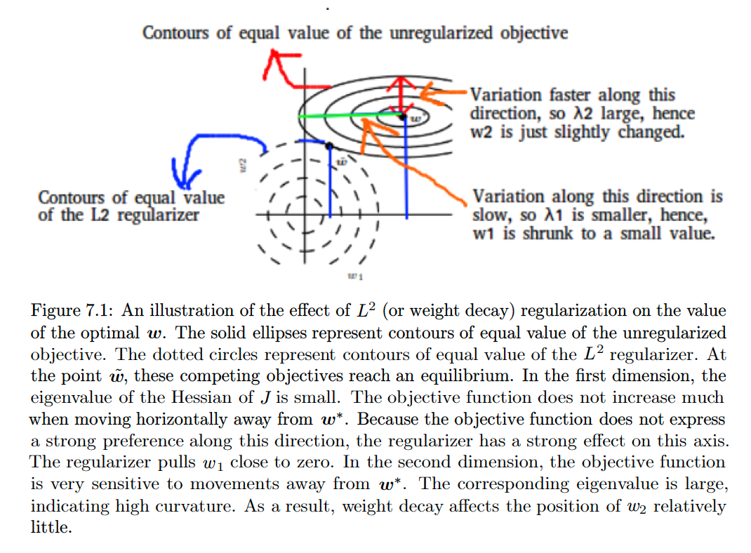
Summary:
Condition Effect of Regularization \(\lambda_{i}>>\alpha\) Not much \(\lambda_{i}<<\alpha\) The weight value almost shrunk to \(0\) - Applying \(L^2\) regularization to Linear Regression :
-
- Weight Decay Analysis (blog)
\(L^2\) Regularization Derivation:
\(L^2\) regularization is equivalent to MAP Bayesian inference with a Gaussian prior on the weights.The MAP Estimate:
$$\begin{aligned} \hat{\theta}_ {\mathrm{MAP}} &=\arg \max_{\theta} P(\theta \vert y) \\ &=\arg \max_{\theta} \frac{P(y \vert \theta) P(\theta)}{P(y)} \\ &=\arg \max_{\theta} P(y \vert \theta) P(\theta) \\ &=\arg \max_{\theta} \log (P(y \vert \theta) P(\theta)) \\ &=\arg \max_{\theta} \log P(y \vert \theta)+\log P(\theta) \end{aligned}$$
We place a Gaussian Prior on the weights, with zero mean and equal variance \(\tau^2\):
$$\begin{aligned} \hat{\theta}_ {\mathrm{MAP}} &=\arg \max_{\theta} \log P(y \vert \theta)+\log P(\theta) \\ &=\arg \max _{\boldsymbol{w}}\left[\log \prod_{i=1}^{n} \dfrac{1}{\sigma \sqrt{2 \pi}} e^{-\dfrac{\left(y_{i}-\boldsymbol{w}^{\top}\boldsymbol{x}_i\right)^{2}}{2 \sigma^{2}}}+\log \prod_{j=0}^{p} \dfrac{1}{\tau \sqrt{2 \pi}} e^{-\dfrac{w_{j}^{2}}{2 \tau^{2}}} \right] \\ &=\arg \max _{\boldsymbol{w}} \left[-\sum_{i=1}^{n} \dfrac{\left(y_{i}-\boldsymbol{w}^{\top}\boldsymbol{x}_i\right)^{2}}{2 \sigma^{2}}-\sum_{j=0}^{p} \dfrac{w_{j}^{2}}{2 \tau^{2}}\right] \\ &=\arg \min_{\boldsymbol{w}} \dfrac{1}{2 \sigma^{2}}\left[\sum_{i=1}^{n}\left(y_{i}-\boldsymbol{w}^{\top}\boldsymbol{x}_i\right)^{2}+\dfrac{\sigma^{2}}{\tau^{2}} \sum_{j=0}^{p} w_{j}^{2}\right] \\ &=\arg \min_{\boldsymbol{w}} \left[\sum_{i=1}^{n}\left(y_{i}-\boldsymbol{w}^{\top}\boldsymbol{x}_i\right)^{2}+\lambda \sum_{j=0}^{p} w_{j}^{2}\right] \\ &= \arg \min_{\boldsymbol{w}} \left[ \|XW - \boldsymbol{y}\|^2 + \lambda {\|\boldsymbol{w}\|_ 2}^2\right]\end{aligned}$$
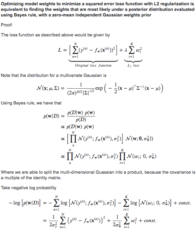
Properties:
- Notice that L2-regularization has a rotational invariance. This actually makes it more sensitive to irrelevant features. [Ref]
- Adding L2-regularization to a convex function gives a strongly-convex function. So L2-regularization can make gradient descent converge much faster. (^ same ref)
Notes:
- L2-reg and Adversarial Examples (New Angle)
- Weight Decay Analysis (blog)
- Interpreting the Penalty term \(\lambda\):
In the Bayesian Interpretation of Weight Decay; by assuming a Gaussian Distribution on the errors:
the Penalty term \(\lambda\) can be interpreted as the (squared) ratio of two variances of the data and the weights respectively: \(\lambda = \frac{\sigma_{D}^{2}}{\sigma_{W}^{2}}\). - A visual explanation for regularization of linear models (Blog)
- What happens in a Single Step:
- \(L^1\) Regularization:
\(L^1\) Regularization is another way to regulate the model by penalizing the size of its parameters; the technique adds a regularization term:$$\Omega(\boldsymbol{\theta})=\|\boldsymbol{w}\|_{1}=\sum_{i}\left|w_{i}\right| \tag{7.18}$$
which is a sum of absolute values of the individual parameters.
The regularized objective function is given by:
$$\tilde{J}(\boldsymbol{w} ; \boldsymbol{X}, \boldsymbol{y})=\alpha\|\boldsymbol{w}\|_ {1}+J(\boldsymbol{w} ; \boldsymbol{X}, \boldsymbol{y}) \tag{7.19}$$
with the corresponding (sub) gradient:
$$\nabla_{\boldsymbol{w}} \tilde{J}(\boldsymbol{w} ; \boldsymbol{X}, \boldsymbol{y})=\alpha \operatorname{sign}(\boldsymbol{w})+\nabla_{\boldsymbol{w}} J(\boldsymbol{X}, \boldsymbol{y} ; \boldsymbol{w}) \tag{7.20}$$
Notice that the regularization contribution to the gradient, no longer scales linearly with each \(w_i\); instead it is a constant factor with a sign = \(\text{sign}(w_i)\).
[Analysis]
Sparsity of the \(L^1\) regularization:
In comparison to \(L^2\), \(L^1\) regularization results in a solution that is more sparse.
The sparsity property has been used extensively as a feature selection mechanism.- LASSO: The Least Absolute Shrinkage and Selection Operator integrates an \(L^1\) penalty with a linear model and a least-squares cost function.
The \(L^1\) penalty causes a subset of the weights to become zero, suggesting that the corresponding features may safely be discarded.
\(L^1\) Regularization Derivation:
\(L^1\) regularization is equivalent to (the log-prior term in) MAP Bayesian inference with an isotropic Laplace distribution prior on the weights:$$\log p(\boldsymbol{w})=\sum_{i} \log \operatorname{Laplace}\left(w_{i} ; 0, \frac{1}{\alpha}\right)=-\alpha\|\boldsymbol{w}\|_ {1}+n \log \alpha-n \log 2 \tag{7.24}$$
note that we can ignore the terms \(\log \alpha-\log 2\) because they do not depend on \(\boldsymbol{w}\).
$$\begin{aligned} \hat{\theta}_ {\mathrm{MAP}} &=\arg \max_{\theta} \log P(y \vert \theta)+\log P(\theta) \\ &=\arg \max _{\boldsymbol{w}}\left[\log \prod_{i=1}^{n} \dfrac{1}{\sigma \sqrt{2 \pi}} e^{-\dfrac{\left(y_{i}-\boldsymbol{w}^{\top}\boldsymbol{x}_i\right)^{2}}{2 \sigma^{2}}}+\log \prod_{j=0}^{p} \dfrac{1}{2 b} e^{-\dfrac{\left|\theta_{j}\right|}{2 b}} \right] \\ &=\arg \max _{\boldsymbol{w}} \left[-\sum_{i=1}^{n} \dfrac{\left(y_{i}-\boldsymbol{w}^{\top}\boldsymbol{x}_i\right)^{2}}{2 \sigma^{2}}-\sum_{j=0}^{p} \dfrac{\left|w_{j}\right|}{2 b}\right] \\ &=\arg \min_{\boldsymbol{w}} \dfrac{1}{2 \sigma^{2}}\left[\sum_{i=1}^{n}\left(y_{i}-\boldsymbol{w}^{\top}\boldsymbol{x}_i\right)^{2}+\dfrac{\sigma^{2}}{b} \sum_{j=0}^{p}\left|w_{j}\right|\right] \\ &=\arg \min_{\boldsymbol{w}} \left[\sum_{i=1}^{n}\left(y_{i}-\boldsymbol{w}^{\top}\boldsymbol{x}_i\right)^{2}+\lambda \sum_{j=0}^{p}\left|w_{j}\right|\right] \\ &= \arg \min_{\boldsymbol{w}} \left[ \|XW - \boldsymbol{y}\|^2 + \lambda \|\boldsymbol{w}\|_ 1\right]\end{aligned}$$
Properties:
- \(L^1\) regularization can occasionally produce non-unique solutions. A simple example is provided in the figure when the space of possible solutions lies on a 45 degree line.
- LASSO: The Least Absolute Shrinkage and Selection Operator integrates an \(L^1\) penalty with a linear model and a least-squares cost function.
-
\(L^1\) VS \(L^2\) Regularization:
- Feature Correlation and Sparsity:
- Identical features:
- \(L^1\) regularization spreads weight arbitrarily (all weights same sign)
- \(L^2\) regularization spreads weight evenly
- Linearly related features:
- \(L^1\) regularization chooses variable with larger scale, \(0\) weight to others
- \(L^2\) prefers variables with larger scale — spreads weight proportional to scale
- Identical features:
Interpreting Sparsity with an Example:
Let’s imagine we are estimating two coefficients in a regression. In \(L^2\) regularization, the solution \(\boldsymbol{w} =(0,1)\) has the same weight as \(\boldsymbol{w}=(\frac{1}{\sqrt{2}}, \frac{1}{\sqrt{2}})\) so they are both treated equally. In \(L^1\) regularization, the same two solutions favor the sparse one:$$\|(1,0)\|_{1}=1<\left\|\left(\frac{1}{\sqrt{2}}, \frac{1}{\sqrt{2}}\right)\right\|_{1}=\sqrt{2}$$
So \(L^2\) regularization doesn’t have any specific built in mechanisms to favor zeroed out coefficients, while \(L^1\) regularization actually favors these sparser solutions.
- Feature Correlation and Sparsity:
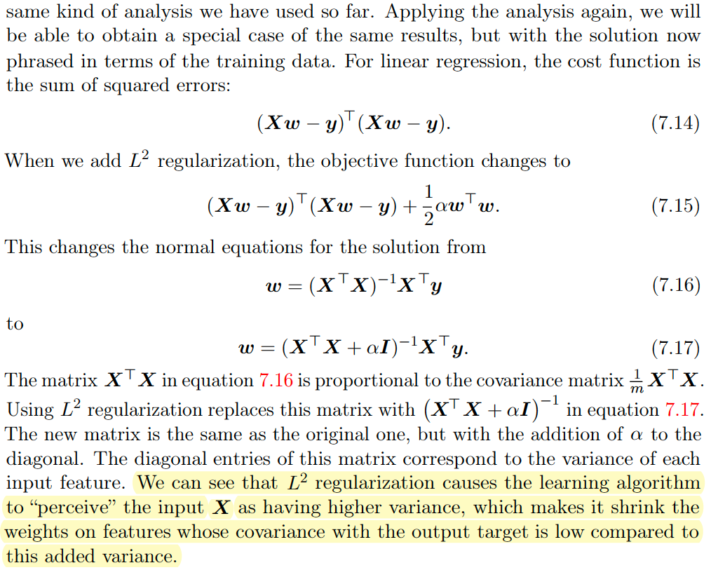
Notes:
- Elastic Net Regularization:
$$\Omega = \lambda\left(\alpha\|w\|_{1}+(1-\alpha)\|w\|_{2}^{2}\right), \alpha \in[0,1]$$
- Combines both \(L^1\) and \(L^2\)
- Used to produce sparse solutions, but to avoid the problem of \(L^1\) solutions being sometimes Non-Unique
- The problem mainly arises with correlated features
- Elastic net regularization tends to have a grouping effect, where correlated input features are assigned equal weights.
-
More generally, we could regularize the parameters to be near any specific point in space and, surprisingly, still get a regularization effect, but better results will be obtained for a value closer to the true one, with zero being a default value that makes sense when we do not know if the correct value should be positive or negative. ↩
-
The approximation is perfect if the objective function is truly quadratic, as in the case of linear regression w/ MSE. ↩