Table of Contents

PyTorch:

CNN Tensor Shape: \([B, C, H, W]\)
CNNs
RNNs
- Modeling Sequences - Memory as a model property:
- Everything:
Memoryless Models for Sequences:- Autoregressive Models:
Predict the next term in a sequence from a fixed number of previous terms using “delay taps”.It tries to predict the next term, basically as a weighted average (if model is linear) of the previous terms.
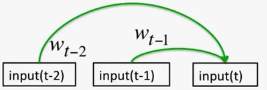
- Feed-Forward Neural Nets:
Generalize Auto-regressive models by using one or more layers of non-linear hidden units e.g. Bengio’s first LM.

Beyond Memoryless Models:
If we give our generative models some hidden state, and if we give this hidden state its own internal dynamics, we get a much more interesting kind of model.
The hidden state produces observations that we get to “observe/see”
- It can store information in its hidden state for a long time.
- If the dynamics is noisy and the way it generates outputs from its hidden state is noisy, (by observing the outputs of the model) we can never know its exact hidden state.
- The best we can do is to infer a probability distribution over the space of hidden state vectors.
- This inference (of the hidden states by observing the outputs of the model) is only tractable for TWO types of hidden-state models:
- Linear Dynamical Systems (LDS) (loved by Engineers):
- These are generative models. They have a real-valued hidden state that cannot be observed directly.
- The hidden state has linear dynamics with Gaussian noise and produces the observations using a linear model with Gaussian noise.
- There may also be driving inputs.
- To predict the next output (so that we can shoot down the missile) we need to infer the hidden state.
- A linearly transformed Gaussian is a Gaussian. So the distribution over the hidden state given the data/observations so far is Gaussian (because all the noise in a LDS is Gaussian). It can be computed using “Kalman filtering”.
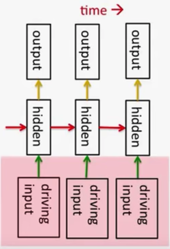
- A linearly transformed Gaussian is a Gaussian. So the distribution over the hidden state given the data/observations so far is Gaussian (because all the noise in a LDS is Gaussian). It can be computed using “Kalman filtering”.
- These are generative models. They have a real-valued hidden state that cannot be observed directly.
- Hidden Markov Models (HMMs) (loved by computer scientists):
- Hidden Markov Models have a discrete one-of-N hidden state distributions (rather than Gaussian distributions). Transitions between states are stochastic and controlled by a transition matrix. The outputs produced by a state are stochastic.
- We cannot be sure which state produced a given output (because the outputs produced by a state are stochastic). So the state is “hidden” (behind this “probabilistic veil”).
- It is easy to represent a probability distribution across N states with N numbers.
So, even tho we cant know what state it is in for sure, we can easily represent the probability distribution
- To predict the next output we need to infer the probability distribution over hidden states.
- HMMs have efficient algorithms for inference and learning (dynamic programming).
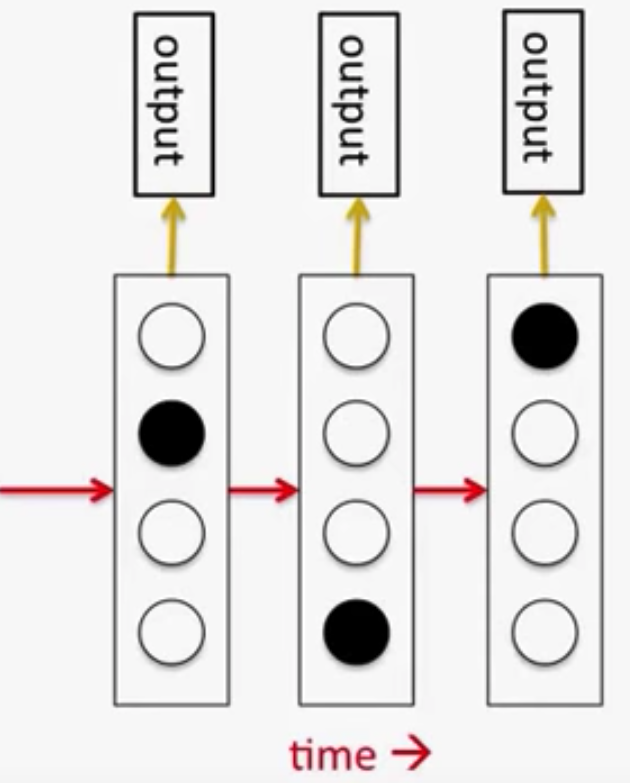
- HMMs have efficient algorithms for inference and learning (dynamic programming).
- A Fundamental Limitation of HMMs:
- Consider what happens when a hidden Markov model generates data
- At each time step it must select one of its hidden states. So with \(N\) hidden states it can only remember \(\log(N)\) bits about what it generated so far.
- Consider the information that the first half of an utterance contains about the second half:
This is the amount of info that the HMM needs to convey to the second half of an utterance it produces from the first half (having produced the first half)
- The syntax needs to fit (e.g. number and tense agreement)
- The semantics needs to fit. The intonation needs to fit.
- The accent, rate, volume, and vocal tract characteristics must all fit.
- All these aspects combined could be \(100\) bits of information that the first half of an utterance needs to convey to the second half. Thus, needing about \(2^100\) hidden states to “remember/store” that information. \(2^100\) is big!
- Consider what happens when a hidden Markov model generates data
- Hidden Markov Models have a discrete one-of-N hidden state distributions (rather than Gaussian distributions). Transitions between states are stochastic and controlled by a transition matrix. The outputs produced by a state are stochastic.
- Linear Dynamical Systems (LDS) (loved by Engineers):
Recurrent Neural Networks (RNNs):
- RNNs are very powerful, because they combine two properties:
- Distributed hidden state that allows them to store a lot of information about the past efficiently.
i.e. several different units can be active at once (unlike HMMs), so they can remember several different things at once.
- Non-linear dynamics that allows them to update their hidden state in complicated ways (unlike LDSs).
- Distributed hidden state that allows them to store a lot of information about the past efficiently.
-
With enough neurons and time, RNNs can compute anything that can be computed by your computer.
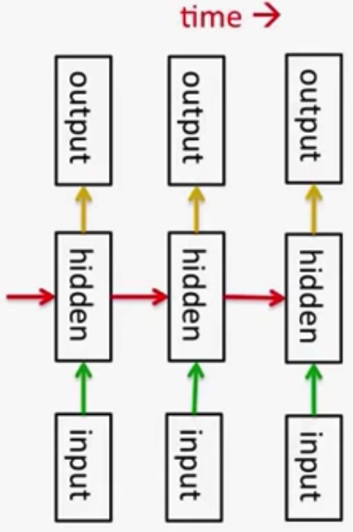
- Visualizing memorization in RNNs
Do generative models need to be stochastic?
-
Linear dynamical systems and HMMs are stochastic models.
The dynamics and the production of observations from the underlying state both involve intrinsic noise.- But the posterior probability distribution over their hidden states given the observed data so far is a deterministic function of the data.
- But the posterior probability distribution over their hidden states given the observed data so far is a deterministic function of the data.
-
Recurrent neural networks are deterministic.
- So think of the hidden state of an RNN as the equivalent of the deterministic probability distribution over hidden states in a linear dynamical system or hidden Markov model.
What kinds of behavior can RNNs exhibit?
- They can oscillate. Good for motor control? (e.g. walking needs varying stride)
- They can settle to point attractors. Good for retrieving memories?
By having the target point-attractors (to settle in) be the memories you want to retrieve.
- They can behave chaotically. Bad for information processing?
- RNNs could potentially learn to implement lots of small programs (using different subsets of their hidden state) that each capture a nugget of knowledge and run in parallel, interacting to produce very complicated effects.
- But the computational power of RNNs makes them very hard to train
- For many years we could not exploit the computational power of RNNs despite some heroic efforts (e.g. Tony Robinson’s speech recognizer)
Notes:
- A Content-Addressable Memory: an item can be accessed by just knowing part of its content.
- Autoregressive Models:
Notes:
- Everything:
- Stability - Vanishing and Exploding Gradients:
Maths
- Metrics and Quasi-Metrics:
- content:
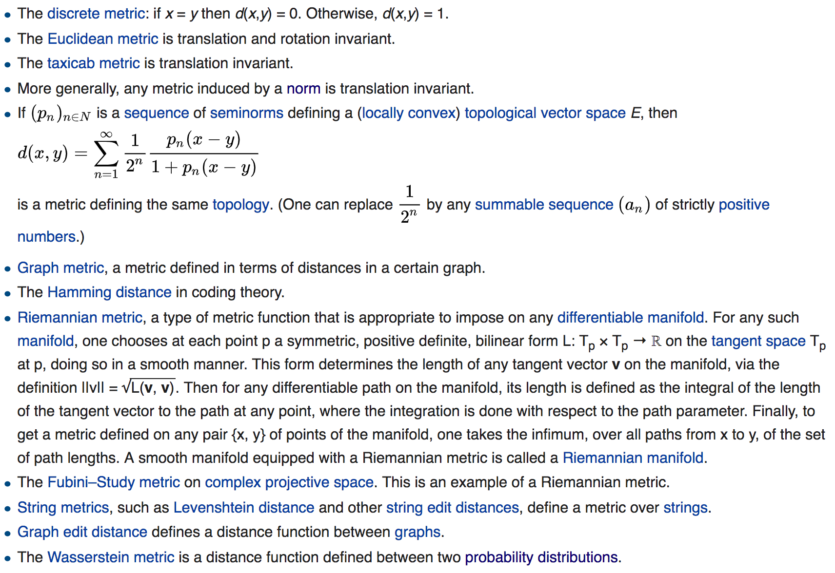
A Metric (distance function) \(d\) is a function that defines a distance between each pair of elements of a set \(X\).
A Metric induces a topology on a set; BUT, not all topologies can be generated by a metric.
Mathematically, it is a function:
\({\displaystyle d:X\times X\to [0,\infty )},\)
that must satisfy the following properties:- \({\displaystyle d(x,y)\geq 0}\) \(\:\:\:\:\:\:\:\) non-negativity or separation axiom
- \({\displaystyle d(x,y)=0\Leftrightarrow x=y}\) \(\:\:\:\:\:\:\:\) identity of indiscernibles
- \({\displaystyle d(x,y)=d(y,x)}\) \(\:\:\:\:\:\:\:\) symmetry
- \({\displaystyle d(x,z)\leq d(x,y)+d(y,z)}\) \(\:\:\:\:\:\:\:\) subadditivity or triangle inequality
The first condition is implied by the others.
A Quasi-Metric is a metric that lacks the symmetry property.
One can form a Metric function \(d'\) from a Quasi-metric function \(d\) by taking:
\(d'(x, y) = 1⁄2(d(x, y) + d(y, x))\)
- content:
- Binary Relations (abstract algebra):
-
content:
A binary relation on a set \(A\) is a set of ordered pairs of elements of \(A\). In other words, it is a subset of the Cartesian product \(A^2 = A ×A\).
The number of binary relations on a set of \(N\) elements is \(= 2^{N^2}\)Examples:
- “is greater than”
- “is equal to”
- A function \(f(x)\)
Properties: (for a relation \(R\) and set \(X\))
- Reflexive: for all \(x\) in \(X\) it holds that \(xRx\)
- Symmetric: for all \(x\) and \(y\) in \(X\) it holds that if \(xRy\) then \(yRx\)
- Transitive: for all \(x\), \(y\) and \(z\) in \(X\) it holds that if \(xRy\) and \(yRz\) then \(xRz\)
An Equivalence Relation has all of the above properties.
-
- Set Theory:
- Number of subsets of a set of \(N\) elements \(= 2^N\)
- Number of pairs (e.g. \((a,b)\)) of a set of \(N\) elements \(= N^2\)
e.g. \(\mathbb{R} \times \mathbb{R} = \mathbb{R}^2\)
- Proof Methods:
- Direct Proof
- Mathematical Induction
- Strong Induction
- Infinite Descent
- Contradiction
- Contraposition (\((p \implies q) \iff (!q \implies !p)\))
- Construction
- Combinatorial
- Exhaustion
- Non-Constructive proof (existence proofs)
- Mathematical Concepts - The Map of Mathematics:
- Real Analysis:
The Real line begets Real Analysis. It’s the study of real numbers and continuous functions on the reals. You have a concrete object (real numbers) and a concrete distance measure (the absolute value function) which is needed for the notions of convergence and continuity. - Metric Spaces:
Less concrete than Real Analysis. You have a numerical way of explaining proximity by a distance measure, and you have a similar way of explaining convergence and continuity. Functional Analysis lies in the middle of those two. - Topology:
Studies topological spaces, WHERE, everything is up for grabs. The proximity measure is no longer numerical. The proximity “measure” around a point is a poset-like at best. This makes the notions of convergence and continuity more tricky. - Functional Analysis:
Can be thought of as a generalization of Linear Algebra to infinite dimensional vector spaces (e.g. spaces of functions with a given property - e.g. continuity). - Differential Topology:
is the study of smooth manifolds and smooth maps. It is fundamentally using tools from calculus (hence the “differential” part in the name) but the focus is on spaces and maps up to diffeomorphism, which means that you don’t care at all about notions like angles, lengths, curvature, flatness etc. Just like in ordinary (non-differential) topology, a gently curved line, a straight line, and a totally squiggly line are all the same up to diffeomorphism (the squiggly line should have no sharp cusps and corners though, which is how this is different from ordinary topology).- Pre-Reqs: include a very good foundation in real analysis, including multivariate differential analysis; linear algebra; and topology.
- Differential Geometry:
Its the study of precisely those things that differential topology doesn’t care about (i.e. angles, curvature, etc.). Here the principal objects of study are manifolds endowed with the much more rigid structure of a (Riemannian) metric, which lets you discuss geometric properties like lengths, angles and curvature.- Applications:
It ties well with: Lie Groups, General Relativity, Symplectic Geometry (Mechanics), Algebraic Topology. - Pre-Reqs: similar to those for Differential Topology: solid multivariate analysis, some topology, and of course linear algebra.
- Applications:
- Algebraic Topology:
the study of algebraic invariants as a tool for classifying topological objects.Some of those invariants can actually be developed via differential topology (de Rham cohomology), but most are defined in completely different terms that do not need the space to have any differential structure whatsoever.
- Pre-Reqs: Hard + Touches a lot of math; topology, a good grounding in algebra (abelian groups, rings etc.), know something about categories and functors.
- Algebraic Geometry:
very different topic. At the most basic level, its the study of algebraic varieties (i.e. sets of solutions to polynomial equations).
Modern algebraic geometry, however, is much wider than this innocent statement seems to imply. It is notoriously complex and requires a very deep understanding of a wide variety of disciplines and domains.- Pre-Reqs: commutative algebra, Galois theory, some number theory (especially algebraic number theory), complex function theory, category theory, and a serving of algebraic topology wouldn’t hurt.
General topology is sort-of required: algebraic geometry uses the notion of “Zariski topology” but, honestly, this topology is so different from the things most analysts and topologists talk about that basic topology won’t help.
- Pre-Reqs: commutative algebra, Galois theory, some number theory (especially algebraic number theory), complex function theory, category theory, and a serving of algebraic topology wouldn’t hurt.
- Real Analysis:
- From Topology to Algebraic Topology:
- Suppose we have a closed loop of rope, i.e., a rope with its ends connected together. Such a closed loop could be a simple ring or it could be knotted up in various different ways:
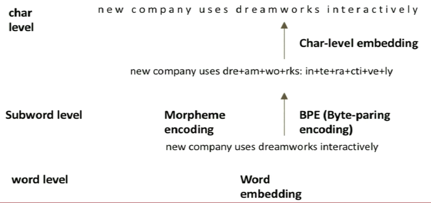
- Now, whether or not it is knotted does not depend on how thick the rope is, how long the rope is, or how it is positioned in space. As long as we don’t cut the rope, any kind of continuous deformation of the rope, such as moving it around, stretching it, bending it, and so on, does not change an unknotted closed loop into a knotted one. So, if we want to study the possible different ways a closed loop can be knotted, we want to ignore any differences related to all these various kinds of continuous deformations. When we ignore all those properties, what is left are called topological properties. So, while two closed loops of different sizes or shapes are geometrically distinct, they could be topologically identical. They are topologically distinct only if they can not be transformed into each other with any continuous deformation. So, in the context of knot theory, topology is the study of the properties of knottedness, which do not depend on the details of position, shape, size, and so on.
- Now, algebraic topology is a way of studying topological properties by translating them into algebraic properties. In the case of knot theory, this might involve, for example, a map that assigns a unique integer to any given closed loop. Such a map can be very useful if we can show that it will always assign the same integer to two closed loops that can be continuously deformed into each other, i.e., topologically equivalent closed loops are always assigned the same number. (Such a map is called a knot invariant.) For example, if we are given two closed loops and they are mapped to different integers, then this instantly tells us that they are topologically distinct from each other. The converse is not necessarily true, since a map with poor “resolving power” might take many topologically distinct closed loops to the same integer. Algebraic topology in the context of knot theory is the study of these kinds of maps from topological objects such as closed loops to algebraic objects such as integers. These maps give, as it were, algebraic perspectives on the topological objects, and that is what algebraic topology in general is about.
- Suppose we have a closed loop of rope, i.e., a rope with its ends connected together. Such a closed loop could be a simple ring or it could be knotted up in various different ways:
- Notes:
- Dot Product Scale/Magnitude: the scale of the dot product increases as dimensions get larger.
Assume that the components of \(q\) and \(k\) are independent random variables with mean \(0\) and variance \(1\). Then their dot product, \(q^Tk = \sum_{i=1}^{d_k} q_ik_i\), (where \(d_k = \vert k \vert\) is the dimension of \(k \in \mathbb{R}^{d_k} \iff q \in \mathbb{R}^{d_q}\)) has mean \(0\) and variance \(d_k\).
- Dot Product Scale/Magnitude: the scale of the dot product increases as dimensions get larger.
- Formulas:
- Binomial Theorem:
$$(x+y)^{n}=\sum_{k=0}^{n}{n \choose k}x^{n-k}y^{k}=\sum_{k=0}^{n}{n \choose k}x^{k}y^{n-k} \\={n \choose 0}x^{n}y^{0}+{n \choose 1}x^{n-1}y^{1}+{n \choose 2}x^{n-2}y^{2}+\cdots +{n \choose n-1}x^{1}y^{n-1}+{n \choose n}x^{0}y^{n},$$
- Binomial Coefficient:
$${\binom {n}{k}}={\frac {n!}{k!(n-k)!}} = {n \text{ choose } k} = {n \choose (n-k)}$$
- Expansion \(x^n - y^n\):
$$x^n - y^n = (x-y)(x^{n-1} + x^{n-2} y + ... + x y^{n-2} + y^{n-1})$$
- Number of subsets of a set of \(N\) elements \(= 2^N\)
- Number of pairs (e.g. \((a,b)\)) of a set of \(N\) elements \(= N^2\)
- Number of subsets of size \(k\) \(= {\binom {n}{k}}\)
- There are at most \(k^N\) ways to partition \(N\) data points into \(k\) clusters - there are \(N\) choose \(k\) clusters, precisely
- Permutations and Combinations:
- Permutations of a set of size \(N\) \(= N!\)

- Permutations of a set of size \(N\) \(= N!\)
- Logarithms:
$$\log_x(y) = \dfrac{\ln(y)}{\ln(x)}$$
- The length of a vector \(\mathbf{x}\) along a direction (projection):
- Along a unit-length vector \(\hat{\mathbf{w}}\): \(\text{comp}_ {\hat{\mathbf{w}}}(\mathbf{x}) = \hat{\mathbf{w}}^T\mathbf{x}\)
- Along an unnormalized vector \(\mathbf{w}\): \(\text{comp}_ {\mathbf{w}}(\mathbf{x}) = \dfrac{1}{\|\mathbf{w}\|} \mathbf{w}^T\mathbf{x}\)
- Summations:
- \[\sum_{i=1}^{n} 2^{i}=2^{n+1}-2\]
- Binomial Theorem:
- Linear Algebra:
Matrices:- Symmetric Matrices:
- can choose its eigenvectors to be orthonormal
- PSD:
- PD:
- Symmetric Matrices:
Statistics and Probability Theory
- ROC Curve:
- A way to quantify how good a binary classifier separates two classes
- True-Positive-Rate / False-Positive-Rate
- Good classifier has a ROC curve that is near the top-left diagonal (hugging it)
- A Bad Classifier has a ROC curve that is close to the diagonal line
- It allows you to set the classification threshold
- You can minimize False-positive rate or maximize the True-Positive Rate
Notes:
- ROC curves (& AUC) are useful even if the predicted probabilities are not “properly calibrated”
- AUC - AUROC:
- Range \(= 0.5 - 1.0\), from poor to perfect
- Range \(= 0.5 - 1.0\), from poor to perfect
-
Statistical Efficiency:
Essentially, a more efficient estimator, experiment, or test needs fewer observations than a less efficient one to achieve a given performance.
Efficiencies are often defined using the variance or mean square error as the measure of desirability.
An efficient estimator is also the minimum variance unbiased estimator (MVUE).- An Efficient Estimator has lower variance than an inefficient one
- The use of an inefficient estimator gives results equivalent to those obtainable from a subset of data; and is therefor, wasteful of data
-
Errors VS Residuals:
The Error of an observed value is the deviation of the observed value from the (unobservable) true value of a quantity of interest.The Residual of an observed value is the difference between the observed value and the estimated value of the quantity of interest.
Notes:
- Why maximize the natural log of the likelihood?:
- Numerical Stability: change products to sums
- The logarithm of a member of the family of exponential probability distributions (which includes the ubiquitous normal) is polynomial in the parameters (i.e. max-likelihood reduces to least-squares for normal distributions)
\(\log\left(\exp\left(-\frac{1}{2}x^2\right)\right) = -\frac{1}{2}x^2\) - The latter form is both more numerically stable and symbolically easier to differentiate than the former. It increases the dynamic range of the optimization algorithm (allowing it to work with extremely large or small values in the same way).
- The logarithm is a monotonic transformation that preserves the locations of the extrema (in particular, the estimated parameters in max-likelihood are identical for the original and the log-transformed formulation)
- (GANs) Sampling from Discrete Distributions | The Gumbel-Softmax Trick
- Covariance Matrix is the inverse of the Metric Tensor
- In Gaussians: \(\Sigma^{1/2}\) maps spheres to ellipsoids; eigenvalues are radii; they are also the standard deviations along the eigenvectors
- Reason we sometimes prefer Biased Estimators:
Mainly, due to the Bias-Variance Decomposition. The MSE takes into account both the bias and the variance and sometimes the biased estimator might have a lower variance than the unbiased one, which results in a total decrease in the MSE. - Cross-Field Terms:
- Independent Variable \(\iff\) Covariate \(\iff\) Feature
- (Collection of) Independent Variables \(\iff\) Covariates \(\iff\) Features \(\iff\) Input
- Dependent Variable \(\iff\) Response \(\iff\) Label \(\iff\) Target \(\iff\) Output
- Statistics VS Machine Learning
- Uncorrelated Features in a Design Matrix:
$$\implies X^TX=nI$$
- Expectation Maximization (EM) Algorithm:
EM-Algo Math
Optimization
-
Sigmoid:
\(\sigma(-x) = 1 - \sigma(x)\) - Gradient-Based Optimization:
Notes:- Gradients can’t propagate through argmax
- Derivative for a max function:
The derivative is defined (even though its not continuous at the threshold) by setting the value at the threshold/zero to be either the right or the left derivative.
This is known as the Sub-Gradient and that’s why gradient descent still works. - Subgradient Descent
- Hessian-Free Optimization | Conjugate Gradient Method (Hinton)
-
Backpropagation:
NOTES:
- Backprop (BPTT specifically here) and concept of Locality:
In this context, local in space means that a unit’s weight vector can be updated using only information stored in the connected units and the unit itself such that update complexity of a single unit is linear in the dimensionality of the weight vector. Local in time means that the updates take place continually (on-line) and depend only on the most recent time step rather than on multiple time steps within a given time horizon as in BPTT. Biological neural networks appear to be local with respect to both time and space. wikipedia - Backpropagation with weight constraints:
- It is easy to modify the backprop algorithm to incorporate linear constraints between the weights.
$$\begin{array}{l}{\text { To constrain: } w_{1}=w_{2}} \\ {\text { we need : } \Delta w_{1}=\Delta w_{2}}\end{array}$$
So, we compute the gradients as usual for each \(w_i\) then average them and update both weights (so they’ll continue to satisfy the constraints).
- It is easy to modify the backprop algorithm to incorporate linear constraints between the weights.
- Backprop is a Leaky Abstraction
- Properties of Loss Functions for Backpropagation:
The mathematical expression of the loss function must fulfill two conditions in order for it to be possibly used in back propagation.[3] The first is that it can be written as an average \({\textstyle E={\frac {1}{n}}\sum _{x}E_{x}}\) over error functions \({\textstyle E_{x}}\) {\textstyle E_{x}}, for \({\textstyle n}\) individual training examples, \({\textstyle x}\). The reason for this assumption is that the backpropagation algorithm calculates the gradient of the error function for a single training example, which needs to be generalized to the overall error function. The second assumption is that it can be written as a function of the outputs from the neural network.
- Backprop (BPTT specifically here) and concept of Locality:
- Error Measures - Loss Functions:
- Cross Entropy:
- Deriving Binary Cross Entropy:
It is the log-likelihood of a Bernoulli probability model.$$\begin{array}{c}{L(p)=p^{y}(1-p)^{1-y}} \\ {\log (L(p))=y \log p+(1-y) \log (1-p)}\end{array}$$
- Cross Entropy > MSE for Classification
- Deriving Binary Cross Entropy:
Notes:
- Loss VS Cost Function:
- Loss is just the Error function from Caltech
- Cost is more general than Loss: usually the sum of all the losses
- Objective function is even more general, but a Cost might be a type of Objective Function
- The Risk Function is an objective function is the expected loss
- Loss Functions for Regression
- MSE:
The principle of mean square error can be derived from the principle of maximum likelihood (after we set a linear model where errors are normally distributed). - Hinge Loss and 0-1 Loss:
- Hinge loss upper bounds 0-1 loss
- It is the tightest convex upper bound on the 0/1 loss
- Minimizing 0-1 loss is NP-hard in the worst-case
img
- Loss functions of common ML models:
- maximize the posterior probabilities (e.g., naive Bayes)
- maximize a fitness function (genetic programming)
- maximize the total reward/value function (reinforcement learning)
- maximize information gain/minimize child node impurities (CART decision tree classification)
- minimize a mean squared error cost (or loss) function (CART, decision tree regression, linear regression, adaptive linear neurons, …
- maximize log-likelihood or minimize cross-entropy loss (or cost) function
- minimize hinge loss (support vector machine)
- Cross Entropy:
- Mathematical Properties, Aspects, Considerations:
- The Composition of Invariant Functions:
A function that is invariant to some transformation (e.g. rotation, permutation, etc.) can be composed by averaging over all transformations (rotations \(\rightarrow\) e.g. rotation invariant filters).
Equivalently, for BoW, we average over all permutations (by averaging the words).
This causes smearing. - Smearing in Invariant Functions:
In the linear case, a rotational invariant function commutes with all rotations of the elements in \(\mathbb{R}\); Any commutative transformation should yield this; or a combo of commutative transformations; thus smearing.Implies that one should not use linear functions to aggregate over the set where we want some transformation invariance
- Permutation Invariance:
- The Weight vector of a linear signal is orthogonal to the decision boundary:
The weight vector \(\mathbf{w}\) is orthogonal to the separating-plane/decision-boundary, defined by \(\mathbf{w}^T\mathbf{x} + b = 0\), in the \(\mathcal{X}\) space; Reason:
Since if you take any two points \(\mathbf{x}^\prime\) and \(\mathbf{x}^{\prime \prime}\) on the plane, and create the vector \(\left(\mathbf{x}^{\prime}-\mathbf{x}^{\prime \prime}\right)\) parallel to the plane by subtracting the two points, then the following equations must hold:$$\mathbf{w}^{\top} \mathbf{x}^{\prime}+b=0 \wedge \mathbf{w}^{\top} \mathbf{x}^{\prime \prime}+b=0 \implies \mathbf{w}^{\top}\left(\mathbf{x}^{\prime}-\mathbf{x}^{\prime \prime}\right)=0$$
Identities:
- Math Identities:
$$\frac{1}{N} \sum_{n=1}^{N}\left(\mathbf{w}^{\mathrm{T}} \mathbf{x}_{n}-y_{n}\right)^{2} = \frac{1}{N}\|\mathrm{Xw}-\mathrm{y}\|^{2}$$
- \(\dfrac{\partial}{\partial y} \vert{x-y}\vert = - \text{sign}(x-y)\)
- \(\dfrac{\partial}{\partial y} \vert{x-y}\vert = - \text{sign}(x-y)\)
Notes:
- The well-behaved property from an optimization standpoint, implies that \(f''(x)\) doesn’t change too much or too rapidly, leading to a nearly quadratic function that is easy to optimize by gradient methods.
- The Composition of Invariant Functions:
- The Method of Lagrange Multipliers:
The constrained optimization problem:$$\min_{\mathbf{x}} f(\mathbf{x}) \text { subject to } g(\mathbf{x}) \leq 0$$
is equivalent to the unconstrained optimization problem:
$$\min_{\mathbf{x}}(f(\mathbf{x})+\lambda g(\mathbf{x}))$$
where \(\lambda\) is a scalar called the Lagrange multiplier.
NOTES:
- Ch.8 Dl-book summary
- Why You Should Use Cross-Entropy Error Instead Of Classification Error Or Mean Squared Error For Neural Network Classifier Training
- Points that satisfy all constraints (i.e. the feasible region) always convex and polytope.
- Optimization Blog on opt techniques
- WHY NORMALIZE THE INPUTS/DATA/SIGNAL
- Optimization by Vector Space Methods (book)
- OLS Derivation and Theory
Machine Learning
- Theory:
- ML from a Probabilistic Approach:
When employing a probabilistic approach to doing “learning” (i.e. choosing the hypothesis), you are trying to find: What is the most probable hypothesis, given the Data.
Why NNs are not enough?
The gist of it is this: neural nets do pattern recognition, which achieves local generalization (which works great for supervised perception). But many simple problems require some (small) amount of abstract modeling, which modern neural nets can’t learn.Is there enough info in the labels to learn good, general features in Classification problems?
(((If the task is to learn to classify a particular image into one class/category; and the categories lie on the same manifold (i.e. just cats and dogs; or just vehicles etc.) then, the model can learn the patterns that relate to the particular class the image belongs to, BUT MOREOVER, it learns to ignore the rest of the patterns (i.e. background). So, in a way, yes, there is no information in the labels that tells the network to learn what a tree is (so any objects in the background are somewhat blurred to the network, they have no higher-order meaning) so the overall higher-level vision capabilities of the network doesn't necessarily "develop".
As for the task of pre-training, we both know that even if you learn the patterns of very specific objects/classes (e.g. cats and dogs) you still need to develop certain visual features (e.g. edge/corner detection) and those featurizers will develop well, regardless of the amount of information. i.e. the lower-level visual capabilities will be developed. (we have evidence that pretraining works really well in Vision).
I think the issue here is with Deterministic Noise (i.e. the Bias of the model). The CNN hypothesis just doesn't do things like inverse graphics and whatnot; regardless of the amount of information.
Finally, a big problem is when the information is just conflicting, like two objects that should be recognized but we only label it as one of them. That's the Stochastic Noise. Which relates directly to how well we would generalize. This can be attributed to many things as well: E.g. (1) One-hot vectors need to be smoothed to allow the network to get a sense of the actual different objects in the image, AND to not over-fit the particulars of the data (e.g. consider a cat that looks like a tiger and a cat that looks like a dog; labeling it with 0.8 cat is much better to learn the "cattiness" of the image than the noise) (2) Target labels are just limited. There aren't enough categories in the target, which puts a huge limitation for one-shot learning generalization)))Neural Tangent Kernel:
NTK Theorem: A properly randomly initialized sufficiently wide deep neural network trained by gradient descent with infinitesimal step size (a.k.a. gradient flow) is equivalent to a kernel regression predictor with a deterministic kernel called neural tangent kernel (NTK).
Thus, As width (of NN) \(\rightarrow \infty\), trajectory approaches the trajectory of GD for a kernel regression problem, where the (fixed) kernel in question is the so-called Neural Tangent Kernel (NTK). (For convolutional nets the kernel is Convolutional NTK or CNTK.)
The paper proves that the evolution of an ANN during training can also be described by a kernel.Analysis and Discussion:
- Start with: Fully-Connected Network, Any Depth, Lipschitz Non-Linearity
- Gather all parameters in the network into one vector \(\theta\): initialized randomly, trained w/ GD
- Since cost is non-convex, the analysis is difficult
- Instead, study the network function \(f_{\theta} : \mathbb{R}^{n_0} \rightarrow \mathbb{R}^{n_L}\) which maps inputs to outputs
We fully characterize the behavior of \(f_{\theta}\) in the infinite-width limit (# of neurons in hidden layer \(\rightarrow \infty\)) - Behavior in the limit of the width:
- In the limit, the network function has a Gaussian distribution at initialization

- The effect of GD on a single point \(\boldsymbol{x}_ 0\) at initialization is to move that point and nearby points slightly

- The difference between the two time-steps results in a smooth spike centered at \(\boldsymbol{x}_ 0\)

- The difference is the same for different initializations.

- As we increase the width of the network, they differences become even more similar

- The behavior is linear i.e. adding another datapoint \(\boldsymbol{x}_ 1\) results in the two spikes being added up

- In the limit, the network function has a Gaussian distribution at initialization
- This behavior in the limit can be nicely described by a kernel.
The Neural Tangent Kernel (NTK):

- Defined: in terms of the derivatives of the function wrt the parameters \(\theta\)
- Describes: how modifying the network function \(f_{\theta}\) at the point \(\boldsymbol{x}\) will influence another point \(\boldsymbol{y}\)
- Properties:
- Finite Width:
Depends on the parameters, thus it is:- Random at initialization
- Time-dependent: varies during training
- Infinite width limit :
$$\theta^{(L)}(x, y) \rightarrow \theta_{\infty}^{(L)}(x, y) \:\: n_i \rightarrow \infty \forall i \in [1, ..., L-1]$$
Independent on the parameters, thus it is:
- Deterministic: converges to a deterministic limit at initialization
- Fixed: its rate of change during training \(\rightarrow 0\)
This explains why the effect of GD was so similar for different initializations.

- Finite Width:
- Now we have all the tools to fully describe the behavior of the network function during training:
- Ex. Least-Squares Regression on 3 points:
- Start w/ random Gaussian Process
- Follow the kernel gradient of the cost wrt NTK
- Ex. Least-Squares Regression on 3 points:
- Kernel GD is simply a generalization of GD to Function Spaces
- Because the cost is convex in function space the function will converge to the minimum if the kernel is Positive Definite
- As width (of NN) \(\rightarrow \infty\), trajectory approaches the trajectory of GD for a kernel regression problem, where the (fixed) kernel in question is the so-called Neural Tangent Kernel (NTK). (For convolutional nets the kernel is Convolutional NTK or CNTK.)
Notes:
- Intuition of why DL Works:
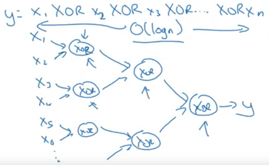
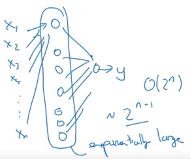
Circuit Theory: There are function you can compute with a “small” L-layer deep NN that shallower networks require exponentially more hidden units to compute. (comes from looking at networks as logic gates).- Example:
Computing \(x_1 \text{XOR} x_2 \text{XOR} ... \text{XOR} x_n\) takes:- \(\mathcal{O}(log(n))\) in a tree representation.
- \(\mathcal{O}(2^n)\) in a one-hidden-layer network because you need to exhaustively enumerate all possible \(2^N\) configurations of the input bits that result in the \(\text{XOR}\) being \({1, 0}\).
- \(\mathcal{O}(log(n))\) in a tree representation.
- Example:
- Curse of Dimensionality (ipynb)
- The Hypothesis space of Neural Networks is Convex:
Composition of affine-relu functions; induction. - Generalization in Deep Learning
- Catastrophic Forgetting:
- mitigating catastrophic forgetting [McCloskey and Cohen, 1989, Ratcliff, 1990, Kemker et al., 2017] by penalizing the norm of parameters when training on a new task [Kirkpatrick et al., 2017], the norm of the difference between parameters for previously learned tasks during parameter updates [Hashimoto et al., 2016], incrementally matching modes [Lee et al., 2017], rehearsing on old tasks [Robins, 1995], using adaptive memory buffers [Gepperth and Karaoguz, 2016], finding task-specific paths through networks [Fernando et al., 2017], and packing new tasks into already trained networks [Mallya and Lazebnik, 2017].
- Overcoming catastrophic forgetting in neural networks (paper)
- ML from a Probabilistic Approach:
-
The Big Formulations:
ML Formulation:
Improve on TASK T with respect to PERFORMANCE METRIC P based on EXPERIENCE E.Problems in ML:
-
T: Categorize email messages as spam or legitimate P: Percentage of email messages correctly classified E: Database of emails, some with human-given labels
-
T: Recognizing hand-written words P: Percentage of words correctly classified E: Database of human-labeled images of handwritten words
-
T: playing checkers P: percentage of games won against an arbitrary opponent E: Playing practice games against itself
- T: Driving on four-lane highways using vision sensors P: Average distance traveled before a human-judged error E: A seq of images and steering commands recorded while observing a human driver
- Sequence Labeling:
- Problems:
- Speech Recognition
- OCR
- Semantic Segmentation
- Approaches:
- CTC - Bi-directional LSTM
- Listen Attend and Spell (LAS)
- HMMs
- CRFs
- Problems:
-
- Types of Learning:
- Multi-Task Learning: general term for training on multiple tasks
- Joint Learning: by choosing mini-batches from two different tasks simultaneously/alternately
- Pre-Training: first train on one task, then train on another
widely used for word embeddings
- Transfer Learning:
a type of multi-task learning where we are focused on one task; by learning on another task then applying those models to our main task - Domain Adaptation:
a type of transfer learning, where the output is the same, but we want to handle different inputs/topics/genres - Zero-Shot Learning:
Notes:
- Relationship between Supervised and Unsupervised Learning:
Many ml algorithms can be used to perform both tasks. E.g., the chain rule of probability states that for a vector \(x \in \mathbb{R}^n\), the joint distribution can be decomposed as:
\(p(\mathbf{x})=\prod_{i=1}^{n} p\left(\mathrm{x}_{i} \vert \mathrm{x}_{1}, \ldots, \mathrm{x}_{i-1}\right)\)
which implies that we can solve the Unsupervised problem of modeling \(p(x)\) by splitting it into \(n\) supervised learning problems.
Alternatively, we can solve the supervised learning problem of learning \(p(y \vert x)\) by using traditional unsupervised learning technologies to learn the joint distribution \(p(x, y)\), then inferring:
\(p(y \vert \mathbf{x})=\frac{p(\mathbf{x}, y)}{\sum_{y} p\left(\mathbf{x}, y^{\prime}\right)}\) - Intuition on Why Unsupervised Learning works:
- Goal: Learn Portuguese
- For 1 month you listen to Portuguese on the radio (this is unlabeled data)
- You develop an intuition for the language, phrases, and grammar (a model in your head)
- It is easier to learn now from a tutor because you have a better (higher representation) of the data/language
- Multi-Task Learning: general term for training on multiple tasks
- Linear Models:
A Linear Model takes an input \(x\) and computes a signal \(s = \sum_{i=0}^d w_ix_i\) that is a linear combination of the input with weights, then apply a scoring function on the signal \(s\).- Linear Classifier as a Parametric Model:
Linear classifiers \(f(x, W)=W x+b\) are an example of a parametric model that sums up the knowledge of the training data in the parameter: weight-matrix \(W\). - Scoring Function:
- Linear Classification:
\(h(x) = sign(s)\) - Linear Regression:
\(h(x) = s\) - Logistic Regression:
\(h(x) = \sigma(s)\)
- Linear Classification:
Notes:
- The Weight vector of a linear signal is orthogonal to the decision boundary:
The weight vector \(\mathbf{w}\) is orthogonal to the separating-plane/decision-boundary, defined by \(\mathbf{w}^T\mathbf{x} + b = 0\), in the \(\mathcal{X}\) space; Reason:
Since if you take any two points \(\mathbf{x}^\prime\) and \(\mathbf{x}^{\prime \prime}\) on the plane, and create the vector \(\left(\mathbf{x}^{\prime}-\mathbf{x}^{\prime \prime}\right)\) parallel to the plane by subtracting the two points, then the following equations must hold:$$\mathbf{w}^{\top} \mathbf{x}^{\prime}+b=0 \wedge \mathbf{w}^{\top} \mathbf{x}^{\prime \prime}+b=0 \implies \mathbf{w}^{\top}\left(\mathbf{x}^{\prime}-\mathbf{x}^{\prime \prime}\right)=0$$
- Linear Classifier as a Parametric Model:
- Bias-Variance Decomposition Theory:
Bias-Variance for Neural-Networks: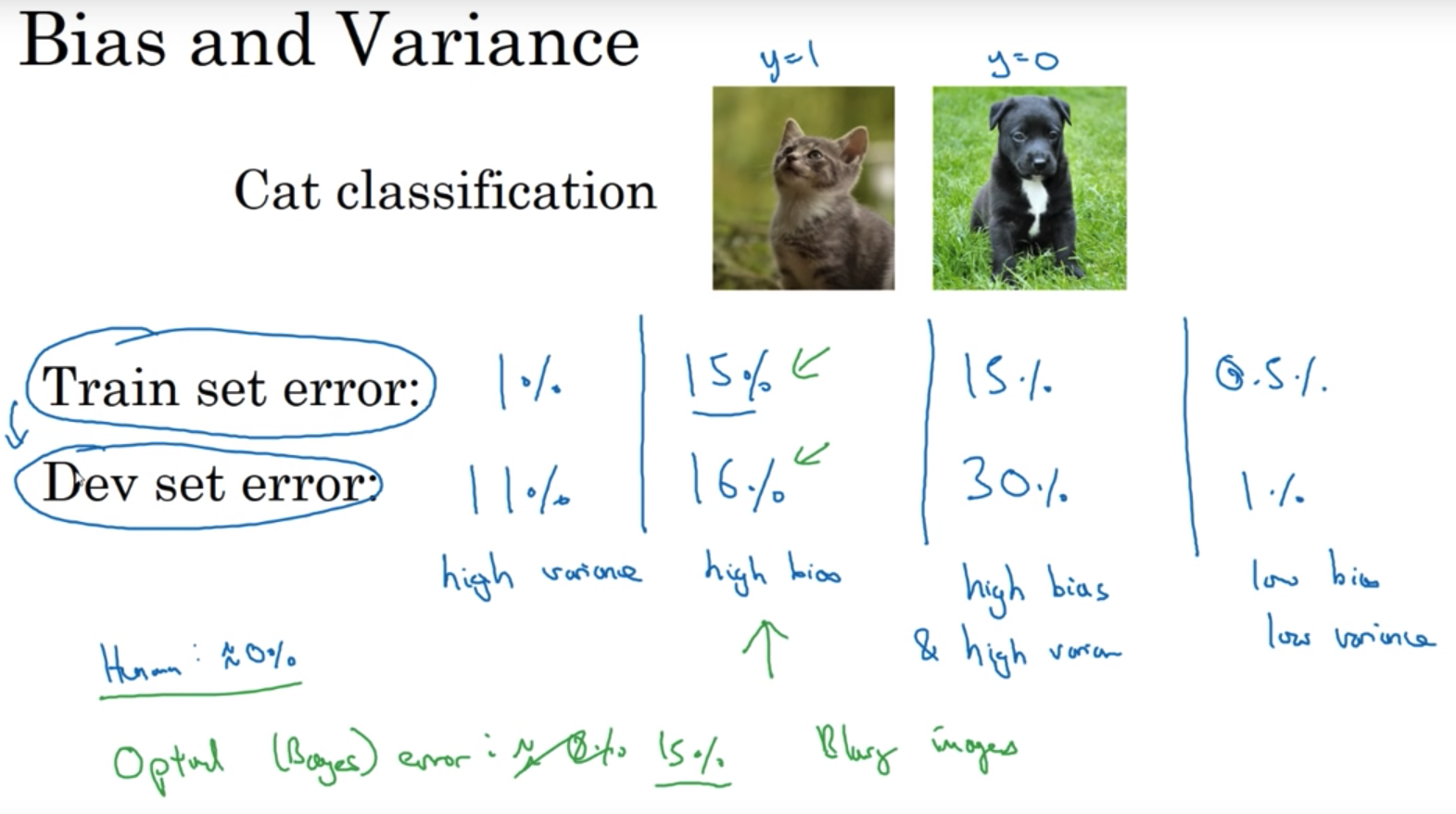
Dealing with Bias and Variance for NN:- High Bias (\(E_{\text{train}}\)) \(\rightarrow\) (1) Bigger Net (2) Train longer (3) Different NN archit
- High Variance (\(E_{\text{dev}}\)) \(\rightarrow\) (1) More Data (2) Regularization (3) Different NN archit
- Models:
Parametric Models:
A parametric model is a set of probability distributions indexed by a parameter \(\theta \in \Theta\). We denote this as:$$\{p(y ; \theta) \vert \theta \in \Theta\},$$
where \(\theta\) is the parameter and \(\Theta\) is the Parameter-Space.
-
Output Units/Functions:
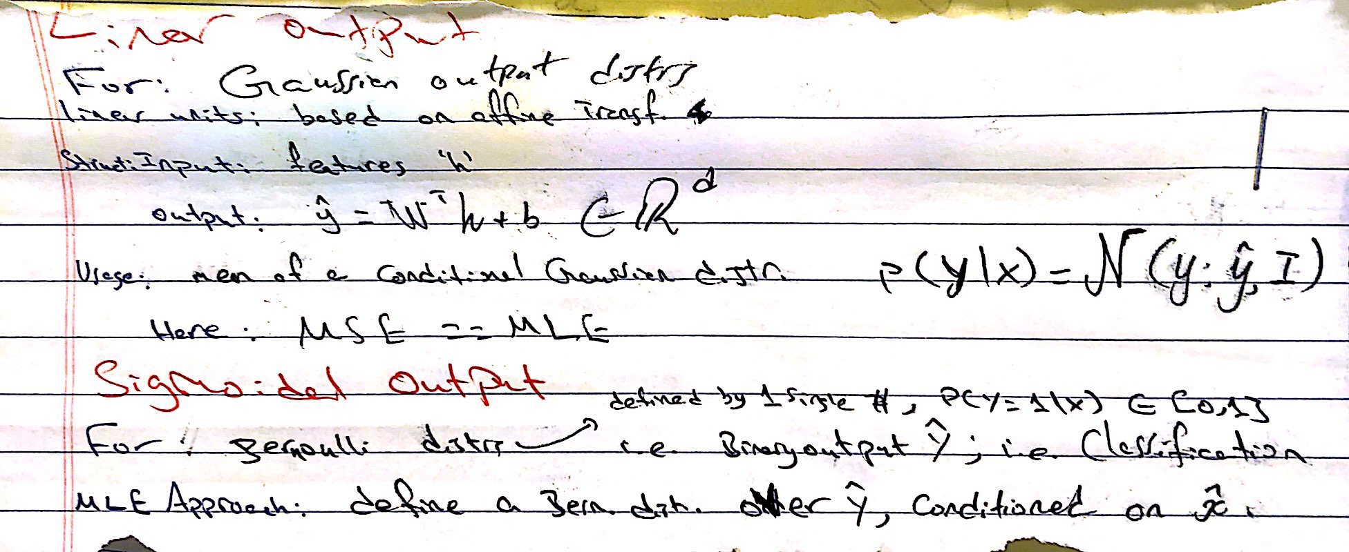
- Model Varieties - Regression and Classification:
Generalized Regression also known as Conditional Distribution Estimation:- Given \(x\), predict probability distribution \(p(y\vert x)\)
- How do we represent the probability distribution?
- We’ll consider parametric families of distributions
- distribution represented by parameter vector
- Examples:
- Generalized Linear Models (GLM)
- Logistic regression (Bernoulli distribution)
- Probit regression (Bernoulli distribution)
- Poisson regression (Poisson distribution)
- Linear regression (Normal distribution, fixed variance)
- Generalized Additive Models (GAM)
- Gradient Boosting Machines (GBM) / AnyBoost
- Generalized Linear Models (GLM)
- We’ll consider parametric families of distributions
Probabilistic Binary Classifiers:
- Setting: \(X=\mathrm{R}^{d}, y=\{0,1\}\)
- For each \(x\), need to predict a distribution on \(y=\{0,1\}\)
- To define a distribution supported on \(\{0,1\}\), it is sufficient to specify the Bernoulli parameter \(\theta=p(y=1 \vert x)\)
- We can refer to this distribution as \(\text{Bernoulli}(\theta)\)
Linear Probabilistic Classifiers:
- Setting: \(X=\mathrm{R}^{d}, y=\{0,1\}\)
- Want prediction function to map each \(x \in \mathrm{R}^{d}\) to the right \(\theta \in[0,1]\)
- We first extract information from \(x \in \mathrm{R}^{d}\) and summarize in a single number
- That number is analogous to the Score in classification
- For a linear method/model, this extraction is done with a linear function;
$$\underbrace{x}_{\in \mathbb{R}^{D}} \mapsto \underbrace{w^{T} x}_{\in \mathrm{R}}$$
- As usual, \(x \mapsto w^{T} x\) will include affine functions if we include a constant features in \(x\)
- \(w^Tx\) is called the linear predictor
- Still need to map this to \([0, 1]\); we do so by Transfer/Response/Inverse-Link function; usually the logistic function (Sigmoid)
Its a function to map the linear predictor in \(\mathbb{R}\) to \([0,1]\):
\(\underbrace{x}_ {\in \mathbf{R}^{D}} \mapsto \underbrace{w^{T}}_{\in R} \mapsto \underbrace{f\left(w^{T} x\right)}_{\in[0,1]}=\theta = p(y=1 \vert x)\)
Learning:
The hypothesis space/set:$$\mathcal{H}=\left\{x \mapsto f\left(w^{T} x\right) \vert w \in \mathbb{R}^{d}\right\}$$
where the only “parameter” in this model is \(w \in \mathbb{R}^d\).
We can choose \(w\) using maximum likelihood:
Likelihood Scoring | Bernoulli Regression:- Suppose we have data \(\mathcal{D}=\left\{\left(x_{1}, y_{1}\right), \ldots,\left(x_{n}, y_{n}\right)\right\}\)
- The model likelihood for \(\mathcal{D}\):
$$\begin{aligned} p_{w}(\mathcal{D}) &=\prod_{i=1}^{n} p_{w}\left(y_{i} \vert x_{i}\right)[\text { by independence }] \\ &=\prod_{i=1}^{n}\left[f\left(w^{T} x_{i}\right)\right]^{y_{i}}\left[1-f\left(w^{T} x_{i}\right)\right]^{1-y_{i}} \end{aligned}$$
- This probability of each data-point \(p_w(y_i\|x_i)\) can be summed in the equation \(\left[f\left(w^{T} x_{i}\right)\right]^{y_{i}}\left[1-f\left(w^{T} x_{i}\right)\right]^{1-y_{i}}\) which capture both cases \(p_w(y_i = 1) = f\left(w^{T} x_{i}\right)\) and \(p_w(y_i = 0) = 1 - f\left(w^{T} x_{i}\right)\)
- The log likelihood:
$$\log p_{w}(\mathcal{D})=\sum_{i=1}^{n} y_{i} \log f\left(w^{T} x_{i}\right)+\left(1-y_{i}\right) \log \left[1-f\left(w^{T} x_{i}\right)\right]$$
- Equivalently, minimize the objective function:
$$J(w)=-\left[\sum_{i=1}^{n} y_{i} \log f\left(w^{T} x_{i}\right)+\left(1-y_{i}\right) \log \left[1-f\left(w^{T} x_{i}\right)\right]\right]$$
Gaussian Linear Regression/Conditional Gaussian Regression:
Generalized Regression as Statistical Learning:
Generalized Linear Models:
- Bayesian Conditional Probabilistic Models:
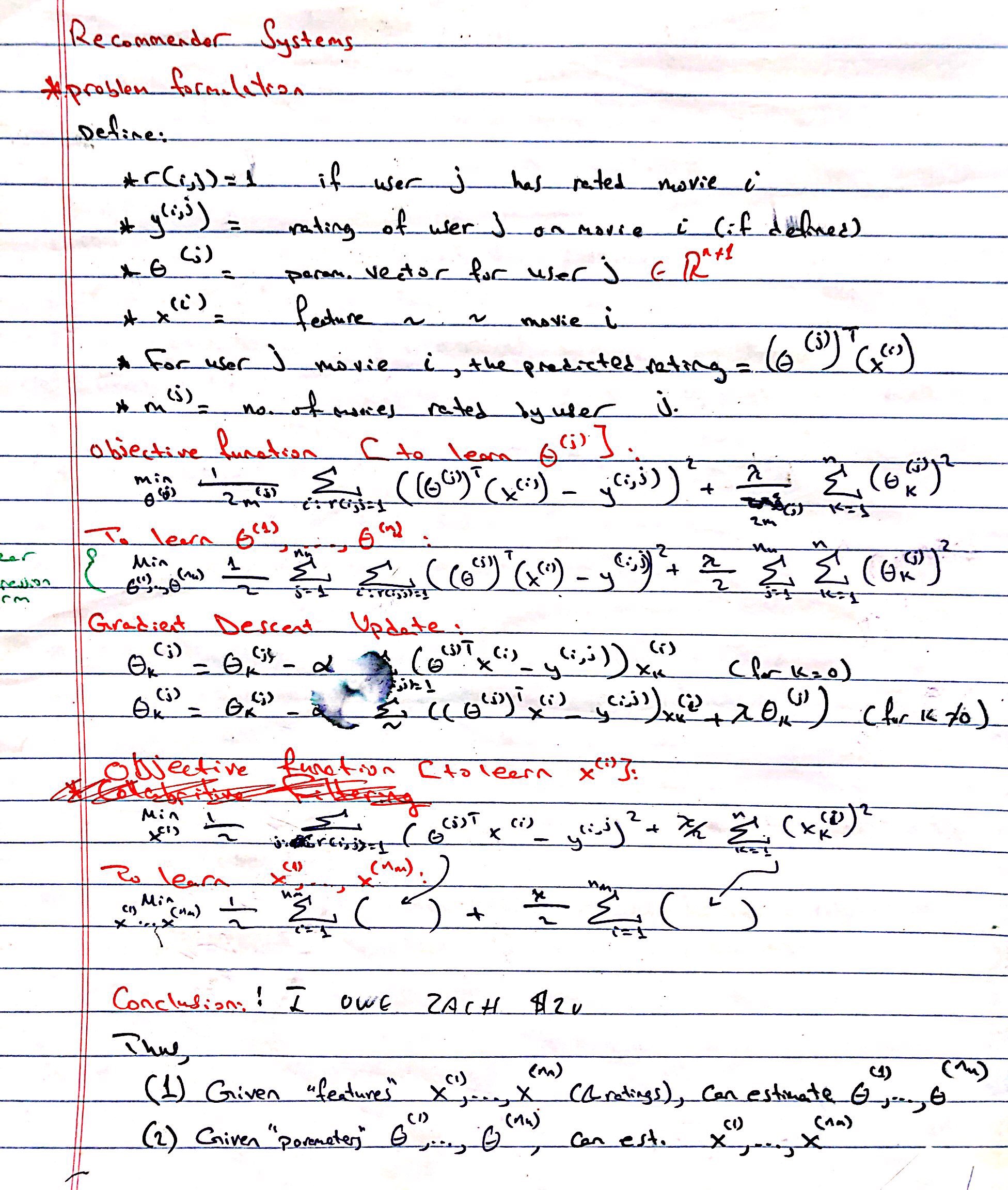
- Recommendation Systems:
- Regularization:
- Overfitting and Regularization:
To address over-fitting:- Increase size of training dataset
- Reduce number of features
- Do Regularization:
- Keep all the features but reduce the magnitude/values of the weights/parameters
- Works well when we have a lot of features, each of which contributes a bit to predicting \(y\)
- Regularization Theory:
- Theoretical Justification for Regularization:
A theoretical justification for regularization is that it attempts to impose Occam’s razor on the solution.
From a Bayesian point of view, many regularization techniques correspond to imposing certain prior distributions on model parameters. - Tikhonov Regularization: is essentially a trade-off between fitting the data and reducing a norm of the solution.
Data Regularization:
- The Design Matrix contains sample points in each row
- Feature Scaling/Mean Normalization (of data):
- Define the mean \(\mu_j\) of each feature of the datapoints \(x^{(i)}\):
$$\mu_{j}=\frac{1}{m} \sum_{i=1}^{m} x_{j}^{(i)}$$
- Replace each \(x_j^{(i)}\) with \(x_j - \mu_j\)
- Centering: subtracting \(\mu\) from each row of \(X\)
- Sphering: applying the transform \(X' = X \Sigma^{-1/2}\)
- Whitening: Centering + Sphering (also known as Decorrelating feature space)
- Overfitting and Regularization:
-
Aggregation - Ensemble Methods:
- Boosting: create different hypothesis \(h_i\)s sequentially + make each new hypothesis decorrelated with previous hypothesis.
- Assumes that this will be combined/ensembled
- Ensures that each new model/hypothesis will give a different/independent output
- Boosting: create different hypothesis \(h_i\)s sequentially + make each new hypothesis decorrelated with previous hypothesis.
- Kernels:
- Kernels:
- Polynomial Kernel of degree, exactly, \(d\):
$$K(\mathbf{u}, \mathbf{v})=(\mathbf{u} \cdot \mathbf{v})^{d}$$
- Polynomial Kernel of degree, up to, \(d\):
$$K(\mathbf{u}, \mathbf{v})=(\mathbf{u} \cdot \mathbf{v}+1)^{d}$$
- Gaussian Kernel:
$$K(\vec{u}, \vec{v})=\exp \left(-\frac{\|\vec{u}-\vec{v}\|_ {2}^{2}}{2 \sigma^{2}}\right)$$
- Sigmoid Kernel:
$$K(\mathbf{u}, \mathbf{v})=\tanh (\eta \mathbf{u} \cdot \mathbf{v}+\nu)$$
- Polynomial Kernel of degree, exactly, \(d\):
- Local Kernels: a kernel where \(k(u, v)\) is large when \(u=v\) and decreases as \(u\) and \(v\) grow further apart from each other.
A local kernel can be thought of as a similarity function that performs template matching, by measuring how closely a test example \(x\) resembles each training example \(x^{(i)}\). -
The kernel trick can NOT be applied to any learning algorithm
- Kernel Regression Introduction
- Kernels:
-
Curse of Dimensionality:
The Curse of Dimensionality, in general, refers to various phenomena, that arise when analyzing and organizing data in high-dimensional spaces, that do not occur in low-dimensional settings such as the three-dimensional physical space of everyday experience.Common Theme:
When the dimensionality increases, the volume of the space increases so fast that the available data become sparse. This sparsity is problematic for any method that requires statistical significance. In order to obtain a statistically sound and reliable result, the amount of data needed to support the result often grows exponentially with the dimensionality. Also, organizing and searching data often relies on detecting areas where objects form groups with similar properties (clustering); in high dimensional data, however, all objects appear to be sparse and dissimilar in many ways, which prevents common data organization strategies from being efficient.Sampling:
The sampling density is proportional to \(N^{1/p}\), where \(p\) is the dimension of the input space and \(N\) is the sample size. Thus, if \(N_1 = 100\) represents a dense sample for a single input problem, then \(N_{10} = 100^{10}\) is the sample size required for the same sampling density with \(10\) inputs. Thus in high dimensions all feasible training samples sparsely populate the input space. - Notes:
- Complexity:
- Caching the activations of a NN:
We need to cache the activation vectors of a NN after each layer \(Z^{[l]}\) because they are required in the backward computation.
- Caching the activations of a NN:
- Initializations:
- Initializing NN:
- Don’t initialize the weights to Zero. The symmetry of hidden units results in a similar computation for each hidden unit, making all the rows of the weight matrix to be equal (by induction).
- It’s OK to initialize the bias term to zero.
- Since a neuron takes the sum of \(N\) inputsXweights, if \(N\) is large, you want smaller \(w_i\)s. You want to initialize with a variance \(\propto \dfrac{1}{n}\) (i.e. multiply by \(\dfrac{1}{\sqrt{n}}\); \(n\) is the number of weights in previous layer).
This doesnt solve but reduces vanishing/exploding gradient problem because \(z\) would take a similar distribution.- Xavier Initialization: assumes \(\tanh\) activation; ^ uses logic above; samples from normal distribution and multiplies by \(\dfrac{1}{\sqrt{n}}\).
- If ReLU activation, it turns out to be better to make variance \(\propto \dfrac{2}{n}\) instead.
- Initializing NN:
- Training:
- Feature Importance:
- In linear models, feature importance can be calculated by the scale of the coefficients
- In tree-based methods (such as random forest), important features are likely to appear closer to the root of the tree. We can get a feature’s importance for random forest by computing the averaging depth at which it appears across all trees in the forest
- Probabilistic Calibration:
- Complexity in ML:
- Definitions of the complexity of an object (\(h\)):
- Minimum Description Length (MDL): the number of bits for specifying an object.
- Order of a Polynomial
- Definitions of the complexity of a class of objects (\(\mathcal{H}\)):
- Entropy
- VC-dim
- Definitions of the complexity of an object (\(h\)):
- Gaussian Discriminant Analysis:
- models $P(Y=y \vert X)$ as a logistic function.
- is a generative model.
- can be used to classify points without ever computing an exponential
- decision boundary shapes:
- Hyperplane
- Nonlinear quadric surface (quadric = the isosurface of a quadratic function)
- The empty set (the classifier always returns the same class)
- Logistic Regression vs LDA? (ESL)
- Geometry of Gaussian Distributions:
- Multivariate Normal Distribution:
- Isotropic:
- I.E. Isosurfaces are spheres
- Covariance Matrix \(\Sigma = \sigma^2 I\)
where \(\sigma^2\) is the variance of any one feature.
- Isotropic:
- Multivariate Normal Distribution:
- The Bias Parameter:
- When is does an ML problem become a Research Problem:
A problem that you are trying to solve using ML becomes a research problem as opposed to those solved by applied practitioners when the only way to learn the problem is to improve the learning algorithm itself. This happens in two situations:- You can fit the training data well but cannot improve generalization error:
This happens when: It is not feasible to gather more data - You cannot fit the training data well even when you increase the capacity of your models as much as you “feasibly” can
- You can fit the training data well but cannot improve generalization error:
-

- Bayesian Deep Learning:
- Uncertainty in deep learning,
- Applications of Bayesian deep learning,
- Probabilistic deep models (such as extensions and application of Bayesian neural networks),
- Deep probabilistic models (such as hierarchical Bayesian models and their applications),
- Generative deep models (such as variational autoencoders),
- Information theory in deep learning,
- Deep ensemble uncertainty,
- NTK and Bayesian modelling,
- Connections between NNs and GPs,
- Incorporating explicit prior knowledge in deep learning (such as posterior regularisation with logic rules),
- Approximate inference for Bayesian deep learning (such as variational Bayes / expectation propagation / etc. in Bayesian neural networks),
- Scalable MCMC inference in Bayesian deep models,
- Deep recognition models for variational inference (amortised inference),
- Bayesian deep reinforcement learning,
- Deep learning with small data,
- Deep learning in Bayesian modelling,
- Probabilistic semi-supervised learning techniques,
- Active learning and Bayesian optimisation for experimental design,
- Kernel methods in Bayesian deep learning,
- Implicit inference,
- Applying non-parametric methods, one-shot learning, and Bayesian deep learning in general.
- Learning Problems:
- Counting/Arithmetic
- Copying
- Identity Mapping
- Pointing (Copying?)
- Learning Features:
- Higher-Order/k-Order Interactions
- Global Dependencies
- Local Dependencies
- Self-Similarity
- Non-Locality (Non-local Neural Networks (paper!))
- Long-Range Dependencies
- Memory: Long-Term, Short-Term (working memory)
- Associative Retrieval
- Mathematical (Symbolic?) Manipulation: Arithmetic?: Counting
- Input Representations:
- Localist Representations
- Point Attractors
- Complexity:
Computer Vision
NLP
The Norvig-Chomsky Debate
Modern Deep Learning Techniques Applied to Natural Language Processing (Amazing Resource)
Deep Learning for NLP: Advancements & Trends
- Language Modeling:
Towards Better Language Modeling (Lec.9 highlight, 38m):To improve a Language Model:
- Better Inputs:
Word \(\rightarrow\) Subword \(\rightarrow\) Char

Subword Language Modeling , Mikolov et al. 2012
Character-Aware Neural Language Model , Kim et al. 2015. - Better Regularization/Preprocessing:
Similar to computer vision, we can do both Regularization and Preprocessing on the data to increase its relevance to the true distribution.
Preprocessing acts as a data augmentation technique. This allows us to achieve a Smoother distribution, since we are removing more common words and re-enforcing rarer words.
Zoneout, Kruger et al. 2016
Data Noising as Smoothing, Xie et al. 2016- Regularization:
- Use Dropout (Zaremba, et al. 2014).
- Use Stochastic FeedForward depth (Huang et al. 2016)
- Use Norm Stabilization (Memisevic 2015) …
- Preprocessing:
- Randomly replacing words in a sentence with other words
- Use bigram statistics to generate Kneser-Ney inspired replacement (Xie et al. 2016).
- Replace a word with fixed drop rate
- Replace a word with adaptive drop rate, by how rare two words appear together (i.e. “Humpty Dumpty”), and replace by a unigram draw over vocab
- Replace a word with adaptive drop rate, and draw word from a proposal distribution (i.e. “New York”)
- Regularization:
- Better Model (+ all above)
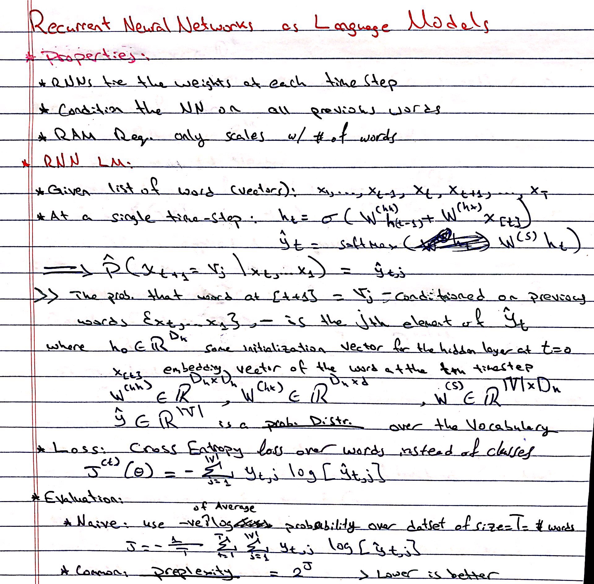
Recurrent Neural Networks as Language Models:
Notes:
- The ML-Estimate of \(p(w_i \vert w_{i-1})\) \(= \dfrac{c(w_{i-1}\:, w_i)}{\sum_{w_i} c(w_{i-1}\:, w_i)}\)
- Better Inputs:
Word \(\rightarrow\) Subword \(\rightarrow\) Char
- Neural Text Generation:
- Traditionally:
- Often Auto-regressive language models (ie. seq2seq)
- These models generate text by sampling words sequentially, with each word conditioned on the previous word
- Benchmarked on validation perplexity even though this is not a direct measure of the quality of the generated text
- The models are typically trained via maximum likelihood and teacher forcing
These methods are well-suited to optimizing perplexity but can result in poor sample quality since generating text requires conditioning on sequences of words that may have never been observed at training time
- Traditionally:
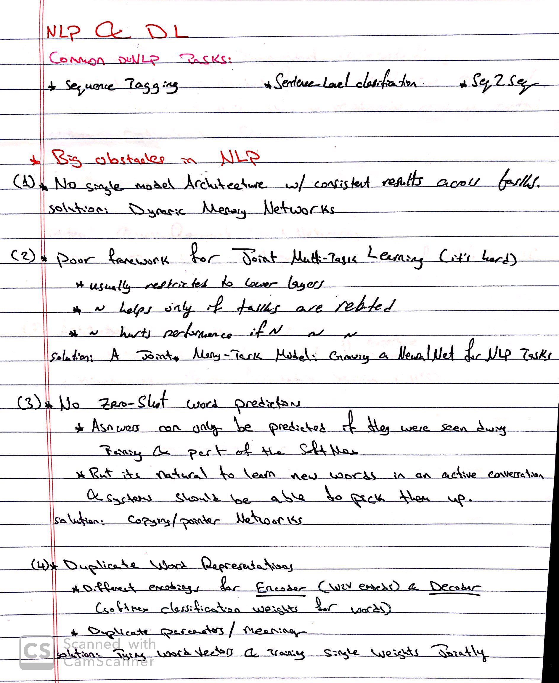
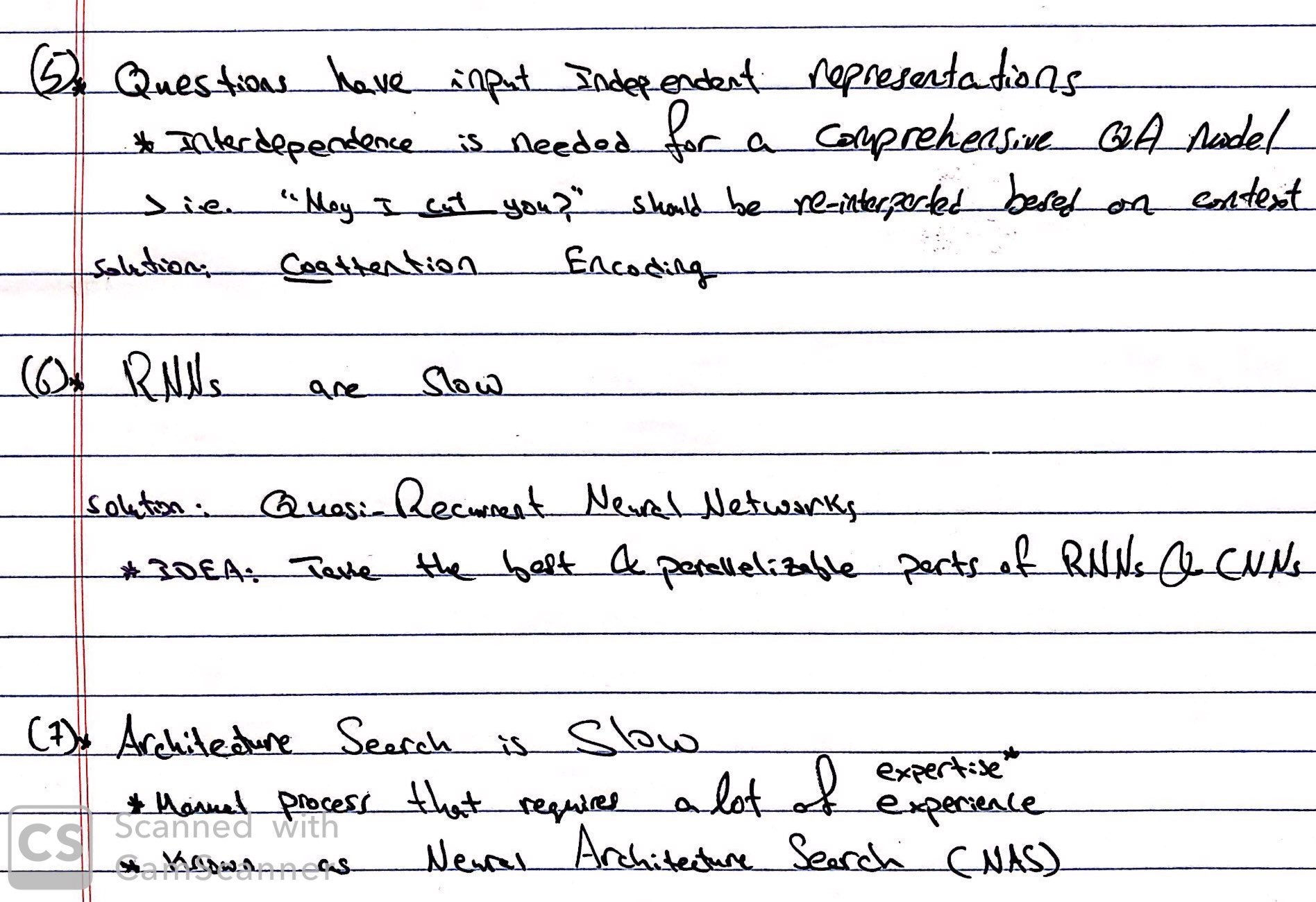
- NLP & DL (R. Sorcher):
-
- Text Classification:
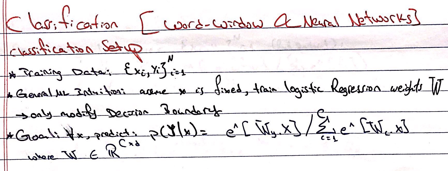
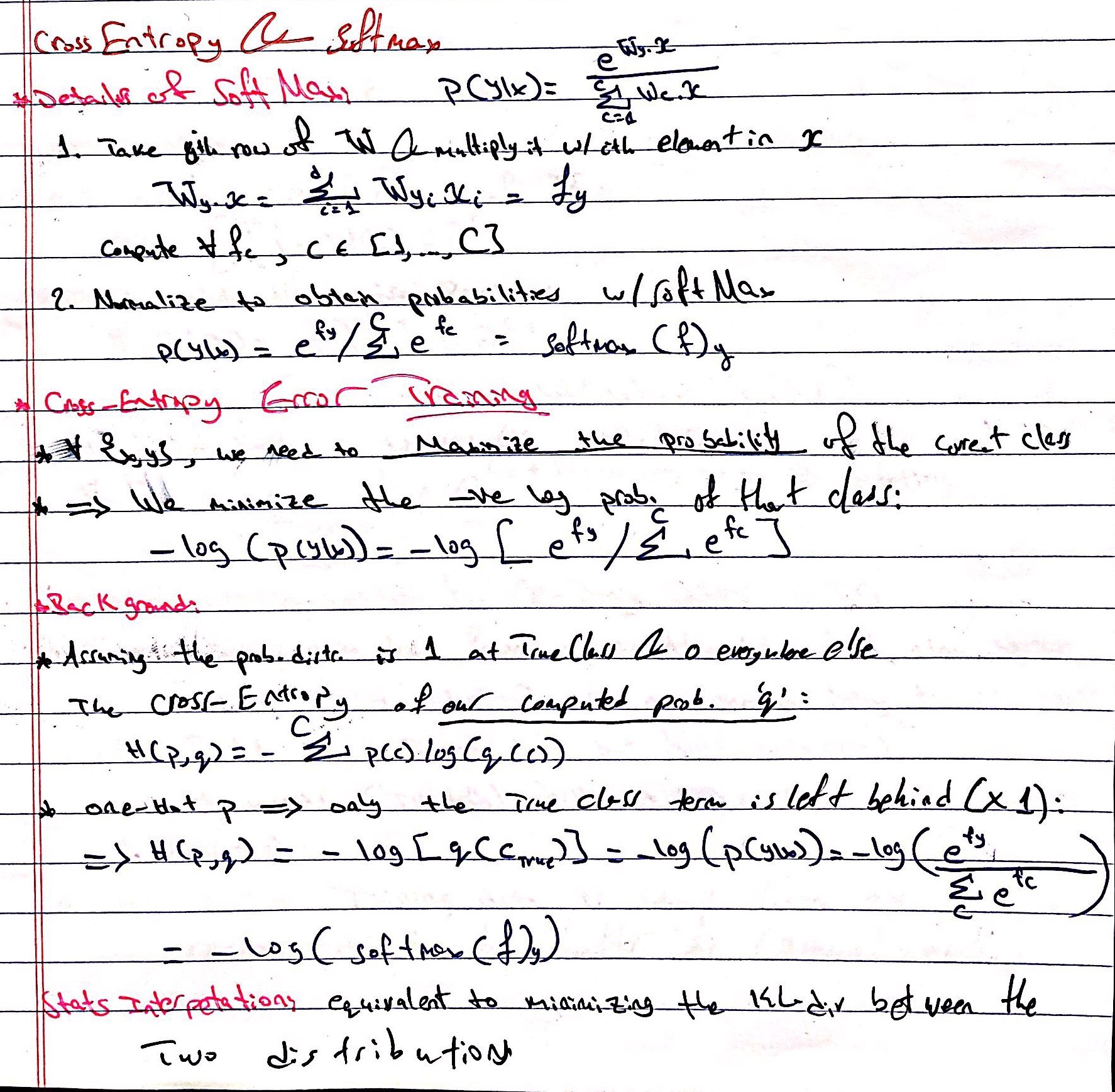
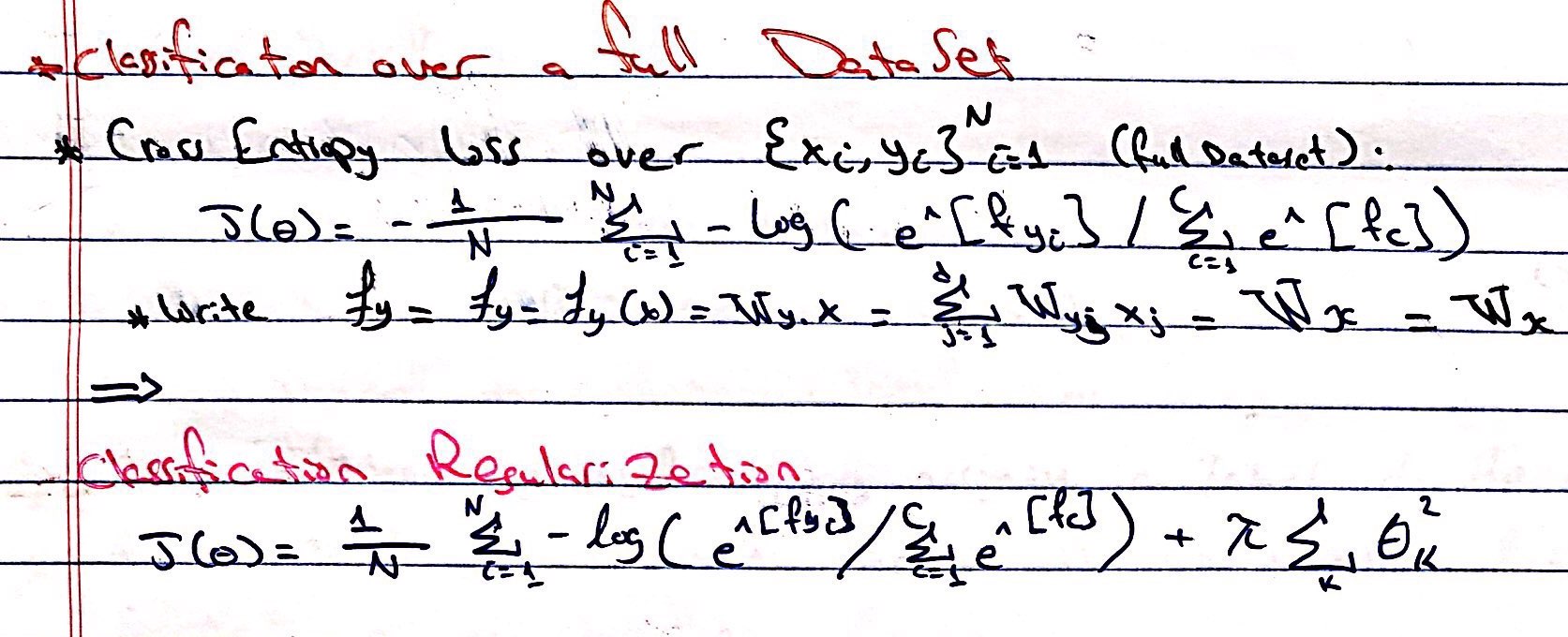
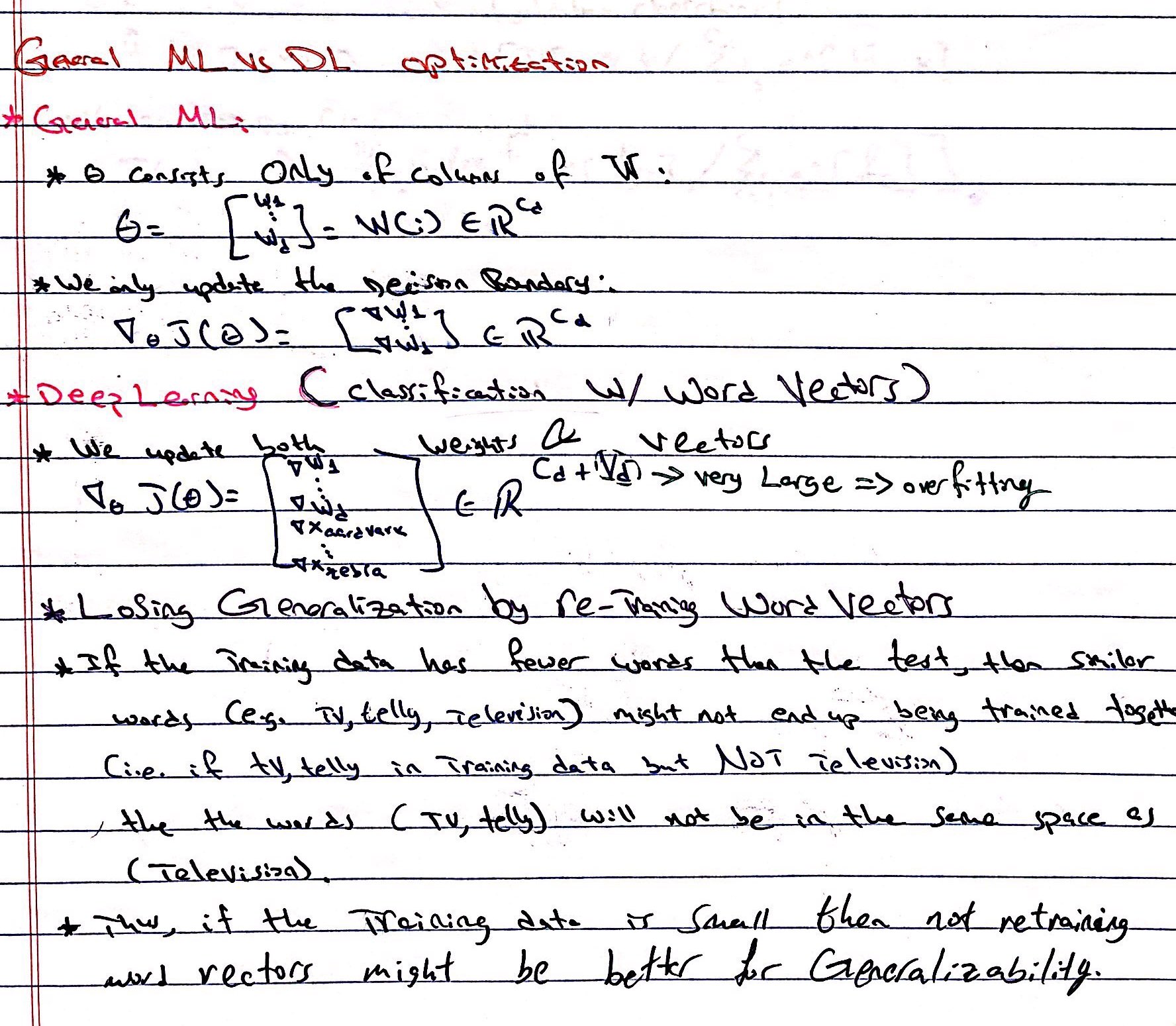
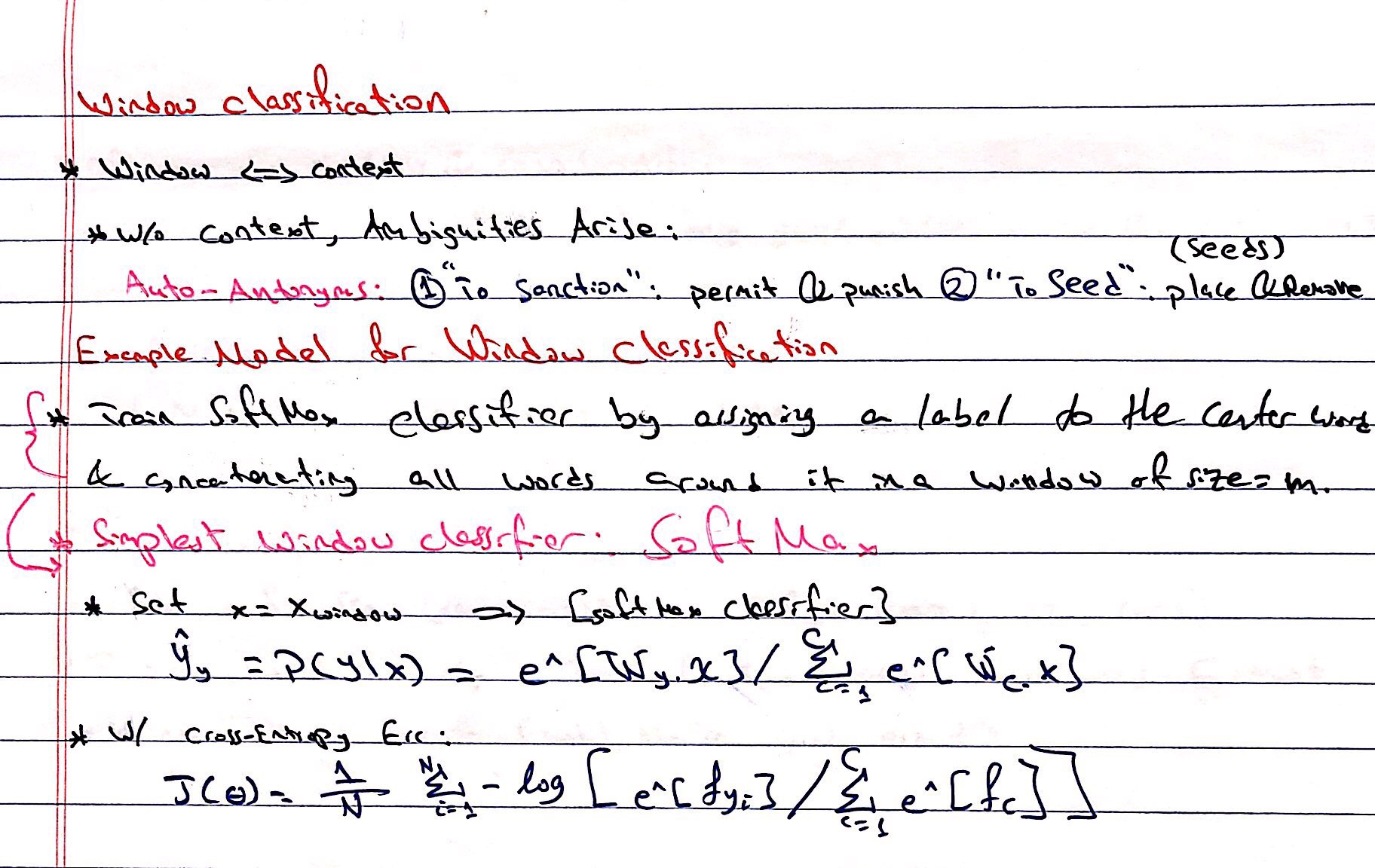
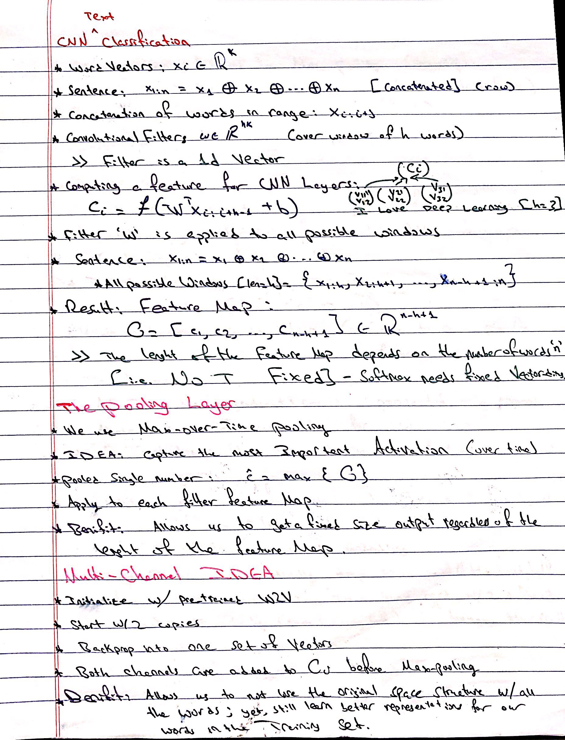
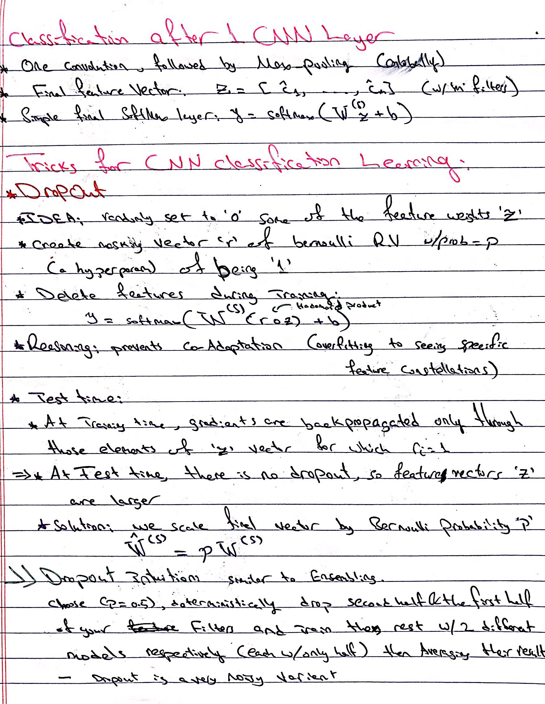
Word-Window Classification:CNN Text Classification:
-
-
Coreference Resolution:
Coreference Resolution: Identify all mentions that refer to the same real world entity.Applications:
- Full text understanding:
- information extraction, question answering, summarization, …
- “He was born in 1961” (Who?)
- Machine Translation:
- languages have different features for gender, number, dropped pronouns, etc.
- Dialogue Systems:
“Book tickets to see James Bond”
“Spectre is playing near you at 2:00 and 3:00 today. How many tickets would you like?”
“Two tickets for the showing at three”
An approach for Coref-Res in 2 steps:
- Detect the Mentions (easy)
“Book tickets to see James Bond”
“Spectre is playing near you at 2:00 and 3:00 today. How many tickets would you like?”
“Two tickets for the showing at three” - Cluster the Mentions (hard)
“Book tickets to see James Bond”
“Spectre is playing near you at 2:00 and 3:00 today. How many tickets would you like?”
“Two tickets for the showing at three”
Mention Detection:
Mention: span of text referring to some entity.Types of Mention:
- Pronouns
“I”, “your”, “it”, “she”, “him” - Named Entities
People, places, etc. - Noun Phrases
“a dog”, “the big fluffy cat stuck in the tree”
Detection:
Use other NLP systems for the detection task:- Pronouns: POS-Tagger
- Named Entities: NER
- Noun Phrases: (Constituency) Parser
Problem with Detection - Extra/bad mentions:
Notice that the systems above will overmatch on possible mentions that don’t have a concrete entity that they refer to: e.g. [It] is sunny, [Every student], [No student], [The best donut in the world], [100 miles].Dealing with bad mentions:
- Train a classifier to filter out spurious mentions
- (more commonly) keep all mentions as “candidate mentions”
- After your coreference system is done running discard all singleton mentions (i.e., ones that have not been marked as coreference with anything else)
- Full text understanding:
- Word Embeddings:
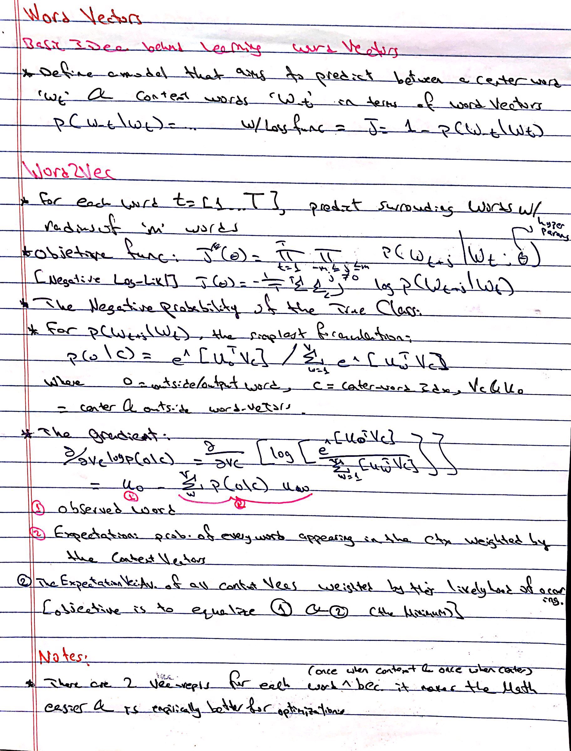
Word Vectors:Notes:
- Categorization is a method for Evaluating w2v Embeddings by creating categorize by clustering, then measuring the purity of the clusters
-
Notes:
- Ilya Sutskever Pubs/Vids
- Can all NLP tasks be cast as QA problems?!
- Survey of the State of the Art in Natural Language Generation
Resources:
- Reinforcement Learning Course Lectures UCL
- Advanced Robotics Lecture CS287 Berk
- Full-Stack DL (productionization of DL) Bootcamp Peter Abbeel
- Deep Unsupervised Learning CS294 Berk
- Deep RL WS1
- Deep RL WS2
- Deep RL Lec CS294 Berk
- DeepLearning Book (dive into dl) Berkeley
- Mathematics of DL
- Deep Learning Linear Algebra
- Intro to Causal Inference (do-Calculus)
- DL and Physics
- EE227C: Convex Optimization and Approximation
- Boyd Cvx-Opt
- Tibshirani Cvx-Opt
- Efficient DL
- Probabilistic Graphical Models CS-708 (CMU!)
- Deep learning courses at UC Berkeley!
- CS182/282A Designing, Visualizing and Understanding Deep Neural Networks Spring 2019
- Quantum Computing Learning Resource (Blog!)
