Data Drift/Shift
- Types of SHIFT:
- Dataset shift happens when the i.i.d. assumptions are not valid for out problem space
- Types of SHIFT:
-
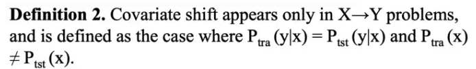
Covariate Shift:
-
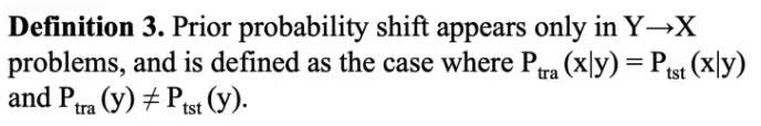
Prior Probability Shift: \(P(x)\)
-
Covariate Shift:
-
Internal CS:
Researchers found that due to the variation in the distribution of activations from the output of a given hidden layer, which are used as the input to a subsequent layer, the network layers can suffer from covariate shift which can impede the training of deep neural networks.-
Covariate shift is the change in the distribution of the covariates specifically, that is, the independent variables. This is normally due to changes in state of latent variables, which could be temporal (even changes to the stationarity of a temporal process), or spatial, or less obvious.
-
IIt introduces BIAS to cross-validation
-
-
The problem of dataset shift can stem from the way input features are utilized, the way training and test sets are selected, data sparsity, shifts in the data distribution due to non-stationary environments, and also from changes in the activation patterns within layers of deep neural networks.
-
- General Data Distribution Shifts:
- Feature change, such as when new features are added, older features are removed, or the set of all possible values of a feature changes: months to years
-
Label schema change is when the set of possible values for Y change. With label shift, P(Y) changes but P(X Y) remains the same. With label schema change, both P(Y) and P(X Y) change. - CREDIT: * With regression tasks, label schema change could happen because of changes in the possible range of label values. Imagine you’re building a model to predict someone’s credit score. Originally, you used a credit score system that ranged from 300 to 850, but you switched to a new system that ranges from 250 to 900.
- Causes of SHIFT:
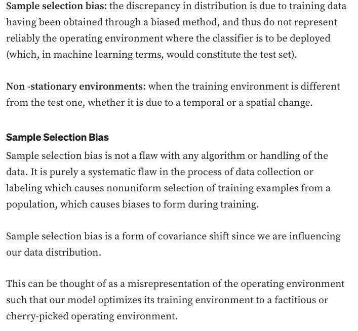
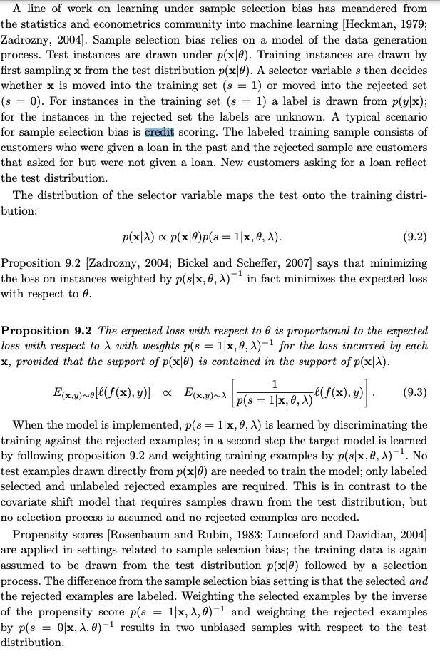
- Dataset shift resulting from sample selection bias is especially relevant when dealing with imbalanced classification, because, in highly imbalanced domains, the minority class is particularly sensitive to singular classification errors, due to the typically low number of samples it presents.
- IN CREDIT
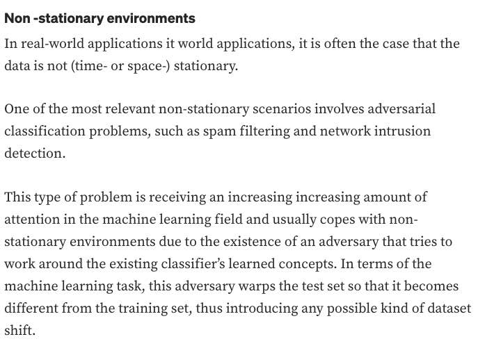
- Non-stationary due to changing macro-economic state
- Adversarial Relationship / Fraud: people might try to game the system to get loans
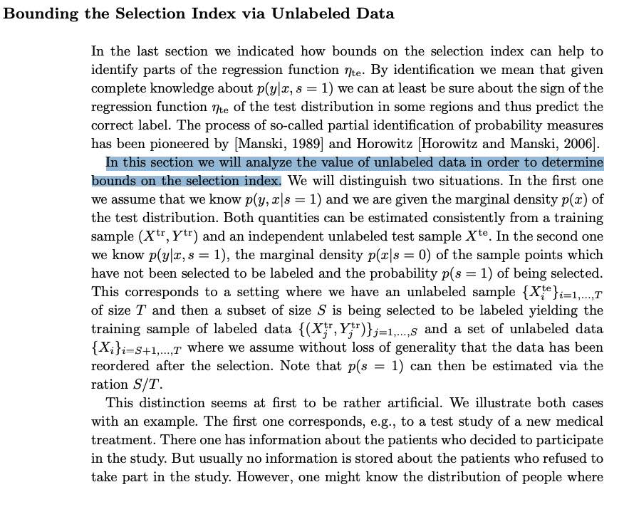
- credit bank has only data from customers whose loan has been approved. This set of customers will be generally a biased sample of the whole population or the set of potential customers.
NEW WORK:
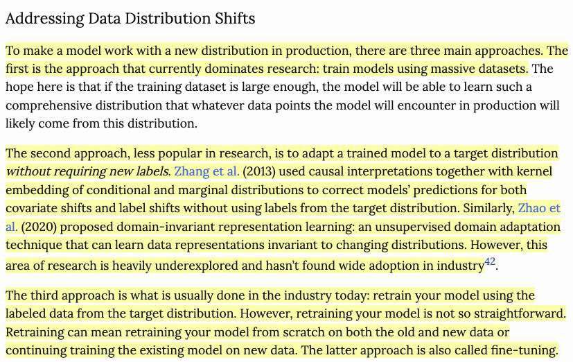
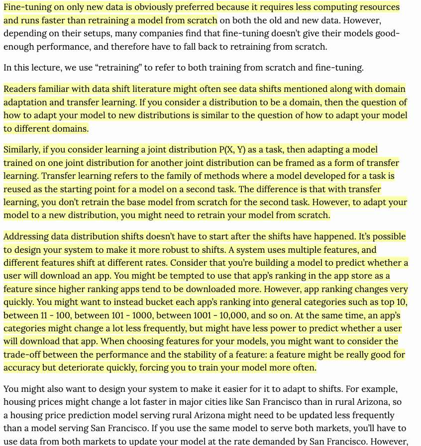
- Handling Data Distribution Shifts:
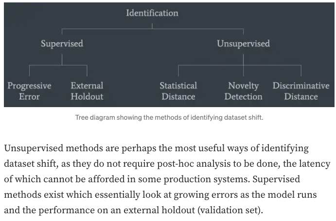
- DETECTION
- HANDLING
- DETECTION:
- monitor your model’s accuracy-related metrics30 in production to see whether they have changed.
-
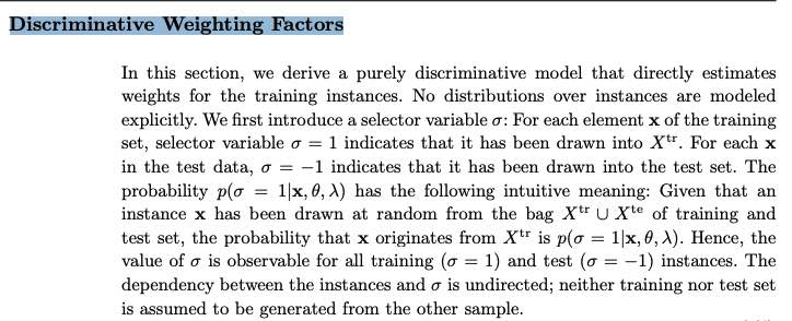
When ground truth labels are unavailable or too delayed to be useful, we can monitor other distributions of interest instead. The distributions of interest are the input distribution P(X), the label distribution P(Y), and the conditional distributions P(X Y) and P(Y X). - In research, there have been efforts to understand and detect label shifts without labels from the target distribution. One such effort is Black Box Shift Estimation by Lipton et al., 2018.
-
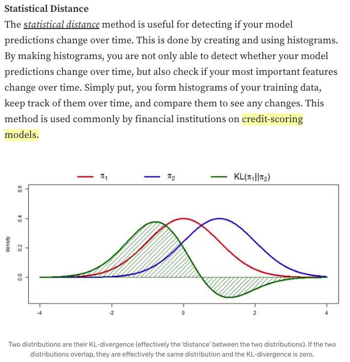
- Statistical Methods:
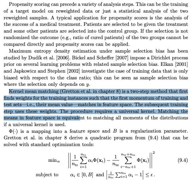
- a simple method many companies use to detect whether the two distributions are the same is to compare their statistics like mean, median, variance, quantiles, skewness, kurtosis, etc. (bad)
- If those metrics differ significantly, the inference distribution might have shifted from the training distribution. However, if those metrics are similar, there’s no guarantee that there’s no shift.
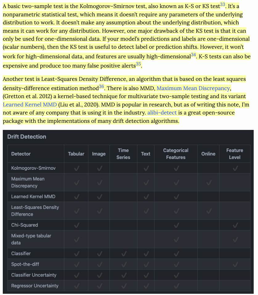
- Because two-sample tests often work better on low-dimensional data than on high-dimensional data, it’s highly recommended that you reduce the dimensionality of your data before performing a two-sample test on them
- a simple method many companies use to detect whether the two distributions are the same is to compare their statistics like mean, median, variance, quantiles, skewness, kurtosis, etc. (bad)
- monitor your model’s accuracy-related metrics30 in production to see whether they have changed.
-
HAndling
- CHip
MONITORING:
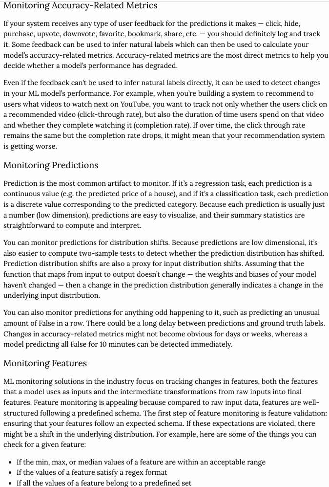
Monitoring Raw Inputs
Encoding
-
Linear Algebra:
-
Linear Algebra:
-
Linear Algebra:
-
Linear Algebra:
Feature Importance
-
Linear Algebra:
-
Linear Algebra:
-
Linear Algebra:
-
Linear Algebra:
Feature Selection
-
Linear Algebra:
-
Linear Algebra:
-
Linear Algebra:
-
Linear Algebra:
Data Preprocessing and Normalization
-
Linear Algebra:
-
Linear Algebra:
Data Regularization:
- The Design Matrix contains sample points in each row
- Feature Scaling/Mean Normalization (of data):
- Define the mean \(\mu_j\) of each feature of the datapoints \(x^{(i)}\):
$$\mu_{j}=\frac{1}{m} \sum_{i=1}^{m} x_{j}^{(i)}$$
- Replace each \(x_j^{(i)}\) with \(x_j - \mu_j\)
- Centering: subtracting \(\mu\) from each row of \(X\)
- Sphering: applying the transform \(X' = X \Sigma^{-1/2}\)
- Whitening: Centering + Sphering (also known as Decorrelating feature space)
Why Normalize the Data/Signal?

-
Linear Algebra:
-
CODE:
Validation & Evaluation - ROC, AUC, Reject Inference + Off-policy Evaluation
-
Linear Algebra:
- ROC:
- A way to quantify how good a binary classifier separates two classes
- True-Positive-Rate / False-Positive-Rate
- Good classifier has a ROC curve that is near the top-left diagonal (hugging it)
- A Bad Classifier has a ROC curve that is close to the diagonal line
- It allows you to set the classification threshold
- You can minimize False-positive rate or maximize the True-Positive Rate
Notes:
- ROC curve is monotone increasing from 0 to 1 and is invariant to any monotone transformation of test results.
- ROC curves (& AUC) are useful even if the predicted probabilities are not “properly calibrated”
- ROC curves are not affected by monotonically increasing functions
- Scale and Threshold Invariance (Blog)
- Accuracy is neither a threshold-invariant metric nor a scale-invariant metric.
-
When to use PRECISION: when data is imbalanced E.G. when the number of negative examples is larger than positive.
Precision does not include TN (True Negatives) so NOT AFFECTED.
In PRACTICE, e.g. studying RARE Disease.
- ROC Curve only cares about the ordering of the scores, not the values.
-
Probability Calibration and ROC: The calibration doesn’t change the order of the scores, it just scales them to make a better match, and the ROC score only cares about the ordering of the scores.
- AUC: The AUC is also the probability that a randomly selected positive example has a higher score than a randomly selected negative example.

-
AUC:
AUC provides an aggregate measure of performance across all possible classification thresholds. One way of interpreting AUC is as the probability that the model ranks a random positive example more highly than a random negative example.-
Range \(= 0.5 - 1.0\), from poor to perfect
- Pros:
- AUC is scale-invariant: It measures how well predictions are ranked, rather than their absolute values.
- AUC is classification-threshold-invariant: It measures the quality of the model’s predictions irrespective of what classification threshold is chosen.
These properties make AUC pretty valuable for evaluating binary classifiers as it provides us with a way to compare them without caring about the classification threshold.
-
Cons
However, both these reasons come with caveats, which may limit the usefulness of AUC in certain use cases:-
Scale invariance is not always desirable. For example, sometimes we really do need well calibrated probability outputs, and AUC won’t tell us about that.
-
Classification-threshold invariance is not always desirable. In cases where there are wide disparities in the cost of false negatives vs. false positives, it may be critical to minimize one type of classification error. For example, when doing email spam detection, you likely want to prioritize minimizing false positives (even if that results in a significant increase of false negatives). AUC isn’t a useful metric for this type of optimization.
-
Notes:
- Partial AUC can be used when only a portion of the entire ROC curve needs to be considered.
-
- Reject Inference and Off-policy Evaluation:
-
Reject inference is a method for performing off-policy evaluation, which is a way to estimate the performance of a policy (a decision-making strategy) based on data generated by a different policy. In reject inference, the idea is to use importance sampling to weight the data in such a way that the samples generated by the behavior policy (the one that generated the data) are down-weighted, while the samples generated by the target policy (the one we want to evaluate) are up-weighted. This allows us to focus on the samples that are most relevant to the policy we are trying to evaluate, which can improve the accuracy of our estimates.
-
Off-policy evaluation is useful in situations where it is not possible or practical to directly evaluate the performance of a policy. For example, in a real-world setting, it may not be possible to directly evaluate a new policy because it could be risky or expensive to implement. In such cases, off-policy evaluation can help us estimate the performance of the policy using data generated by a different, perhaps safer or more easily implemented, policy.
-
-
Validation:
-
Validate a model with given constraints (see above).
Spoke to the recruiter who was super nice and transparent. Scheduled a technical screening afterwards. The question was to validate a model only knowing the true values and predicted values. The interviewer wanted to incorporate the business value of the model. I found this to be interesting and odd as how can the business value validate any model. As we walked through the problem, the interviewer did not care about traditional statistical error measures and techniques in model validation. The interviewer wanted to incorporate the business cases (i.e. total loss in revenue and gains) to validate the model. To me, it felt more business intelligence rather than traditional statistics/machine learning model validation. I am uncertain if data scientists at Affirm are just BI with Python skills.
-
- Evaluation:
- Precision vs Recall Tradeoff:
-
Recall is more important where Overlooked Cases (False Negatives) are more costly than False Alarms (False Positive). The focus in these problems is finding the positive cases.
-
Precision is more important where False Alarms (False Positives) are more costly than Overlooked Cases (False Negatives). The focus in these problems is in weeding out the negative cases.
-
- Precision vs Recall Tradeoff:
Regularization
-
Regularization:
-
Norms:
-
AUC:
-
Linear Algebra:
Interpretability
-
Regularization:
-
Norms:
-
AUC:
-
Linear Algebra:
Decision Trees, Random Forests, XGB, and Gradient Boosting
-
Regularization:
-
Norms:
-
AUC:
-
Boosting:
-
Boosting:
- Boosting: create different hypothesis \(h_i\)s sequentially + make each new hypothesis decorrelated with previous hypothesis.
- Assumes that this will be combined/ensembled
- Ensures that each new model/hypothesis will give a different/independent output
- Boosting: create different hypothesis \(h_i\)s sequentially + make each new hypothesis decorrelated with previous hypothesis.
Uncertainty and Probabilistic Calibration
- Uncertainty:
- Aleatoric vs Epistemic:
Aleatoric uncertainty and epistemic uncertainty are two types of uncertainty that can arise in statistical modeling and machine learning. Aleatoric uncertainty is a type of uncertainty that arises from randomness or inherent noise in the data. It is inherent to the system being studied and cannot be reduced through additional data or better modeling. On the other hand, epistemic uncertainty is a type of uncertainty that arises from incomplete or imperfect knowledge about the system being studied. It can be reduced through additional data or better modeling.
- Aleatoric vs Epistemic:
-
Model Uncertainty, Softmax, and Dropout:
Interpreting Softmax Output Probabilities:
Softmax outputs only measure Aleatoric Uncertainty.
In the same way that in regression, a NN with two outputs, one representing mean and one variance, that parameterise a Gaussian, can capture aleatoric uncertainty, even though the model is deterministic.
Bayesian NNs (dropout included), aim to capture epistemic (aka model) uncertainty.Dropout for Measuring Model (epistemic) Uncertainty:
Dropout can give us principled uncertainty estimates.
Principled in the sense that the uncertainty estimates basically approximate those of our Gaussian process.Theoretical Motivation: dropout neural networks are identical to variational inference in Gaussian processes.
Interpretations of Dropout:- Dropout is just a diagonal noise matrix with the diagonal elements set to either 0 or 1.
- What My Deep Model Doesn’t Know (Blog! - Yarin Gal)
- Calibration in Deep Networks:
- Linear Algebra:
Extra: Bandit, bootstrapping, and prediction interval estimation, Linear Models in Credit
-
Bandit:
-
bootstrapping:
-
prediction interval estimation:
-
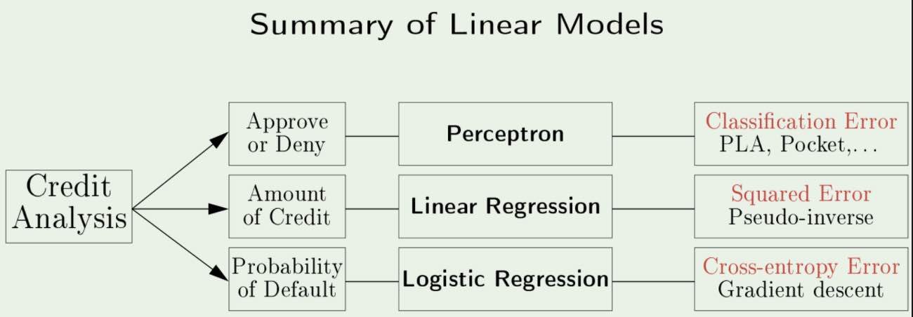
Linear Models in Credit Analysis:
 s
s -
Errors vs Residuals:
The Error of an observed value is the deviation of the observed value from the (unobservable) true value of a quantity of interest.The Residual of an observed value is the difference between the observed value and the estimated value of the quantity of interest.
Notes from Affirm Blog
-
Bandit:
-
bootstrapping:
-
prediction interval estimation:
-
Linear Models in Credit Analysis:
s