- List limitations of PCA:
- PCA is highly sensitive to the (relative) scaling of the data; no consensus on best scaling.
- Feature Importance
- Use linear regression and select variables based on \(p\) values
- Use Random Forest, Xgboost and plot variable importance chart
- Lasso
- Measure information gain for the available set of features and select top \(n\) features accordingly.
- Use Forward Selection, Backward Selection, Stepwise Selection
- Remove the correlated variables prior to selecting important variables
- In linear models, feature importance can be calculated by the scale of the coefficients
- In tree-based methods (such as random forest), important features are likely to appear closer to the root of the tree. We can get a feature’s importance for random forest by computing the averaging depth at which it appears across all trees in the forest
-
Define Relative Entropy - Give it’s formula:
The Kullback–Leibler divergence (Relative Entropy) is a measure of how one probability distribution diverges from a second, expected probability distribution.Mathematically:
$${\displaystyle D_{\text{KL}}(P\parallel Q)=\operatorname{E}_{x \sim P} \left[\log \dfrac{P(x)}{Q(x)}\right]=\operatorname{E}_{x \sim P} \left[\log P(x) - \log Q(x)\right]}$$
- Discrete:
$${\displaystyle D_{\text{KL}}(P\parallel Q)=\sum_{i}P(i)\log \left({\frac {P(i)}{Q(i)}}\right)}$$
- Continuous:
$${\displaystyle D_{\text{KL}}(P\parallel Q)=\int_{-\infty }^{\infty }p(x)\log \left({\frac {p(x)}{q(x)}}\right)\,dx,}$$
- Give an interpretation:
- Discrete variables:
It is the extra amount of information needed to send a message containing symbols drawn from probability distribution \(P\), when we use a code that was designed to minimize the length of messages drawn from probability distribution \(Q\).
- Discrete variables:
- List the properties:
- Non-Negativity:
\({\displaystyle D_{\mathrm {KL} }(P\|Q) \geq 0}\) - \({\displaystyle D_{\mathrm {KL} }(P\|Q) = 0 \iff}\) \(P\) and \(Q\) are:
- Discrete Variables:
the same distribution - Continuous Variables:
equal “almost everywhere”
- Discrete Variables:
- Additivity of Independent Distributions:
\({\displaystyle D_{\text{KL}}(P\parallel Q)=D_{\text{KL}}(P_{1}\parallel Q_{1})+D_{\text{KL}}(P_{2}\parallel Q_{2}).}\) - \({\displaystyle D_{\mathrm {KL} }(P\|Q) \neq D_{\mathrm {KL} }(Q\|P)}\)
This asymmetry means that there are important consequences to the choice of the ordering
- Convexity in the pair of PMFs \((p, q)\) (i.e. \({\displaystyle (p_{1},q_{1})}\) and \({\displaystyle (p_{2},q_{2})}\) are two pairs of PMFs):
\({\displaystyle D_{\text{KL}}(\lambda p_{1}+(1-\lambda )p_{2}\parallel \lambda q_{1}+(1-\lambda )q_{2})\leq \lambda D_{\text{KL}}(p_{1}\parallel q_{1})+(1-\lambda )D_{\text{KL}}(p_{2}\parallel q_{2}){\text{ for }}0\leq \lambda \leq 1.}\)
- Non-Negativity:
- Describe it as a distance:
Because the KL divergence is non-negative and measures the difference between two distributions, it is often conceptualized as measuring some sort of distance between these distributions.
However, it is not a true distance measure because it is not symmetric.KL-div is, however, a Quasi-Metric, since it satisfies all the properties of a distance-metric except symmetry
- List the applications of relative entropy:
Characterizing:- Relative (Shannon) entropy in information systems
- Randomness in continuous time-series
- Information gain when comparing statistical models of inference
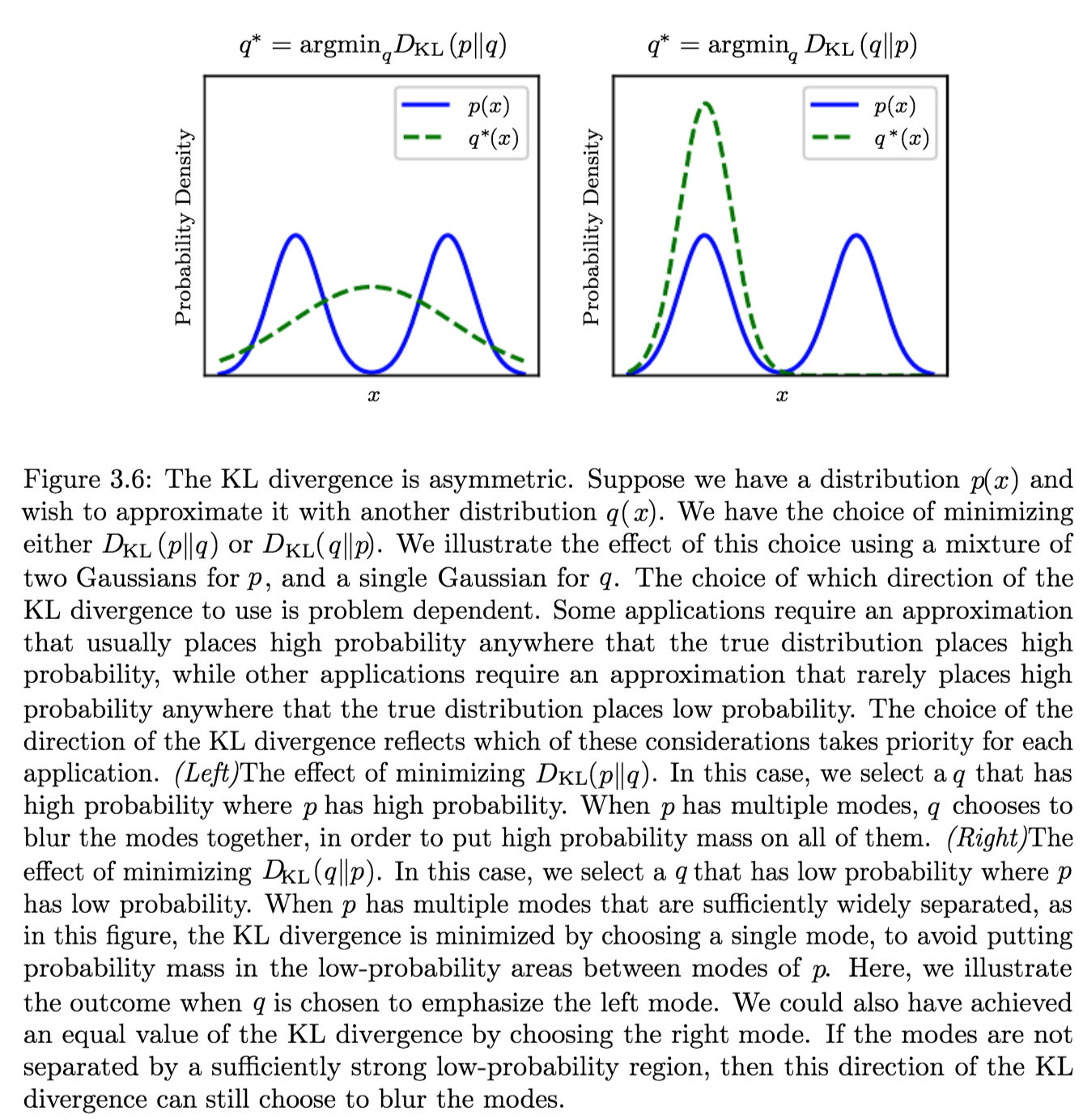
- How does the direction of minimization affect the optimization:
Suppose we have a distribution \(p(x)\) and we wish to approximate it with another distribution \(q(x)\).
We have a choice of minimizing either:- \({\displaystyle D_{\text{KL}}(p\|q)} \implies q^\ast = \operatorname {arg\,min}_q {\displaystyle D_{\text{KL}}(p\|q)}\)
Produces an approximation that usually places high probability anywhere that the true distribution places high probability. - \({\displaystyle D_{\text{KL}}(q\|p)} \implies q^\ast \operatorname {arg\,min}_q {\displaystyle D_{\text{KL}}(q\|p)}\)
Produces an approximation that rarely places high probability anywhere that the true distribution places low probability.which are different due to the asymmetry of the KL-divergence
- \({\displaystyle D_{\text{KL}}(p\|q)} \implies q^\ast = \operatorname {arg\,min}_q {\displaystyle D_{\text{KL}}(p\|q)}\)