Linear Functions and Transformations, and Maps

1. Linear Functions:

   Linear functions are functions which preserve scaling and addition of the input argument.

   Formally,

   A function $f: \mathbf{R}^n \rightarrow \mathbf{R}$ is linear if and only if $f$ preserves scaling and addition of its arguments:

   • for every $x \in \mathbf{R}^n$, and $\alpha \in \mathbf{R}, \ f(\alpha x) = \alpha f(x)$; and

   • for every $x_1, x_2 \in \mathbf{R}^n, f(x_1+x_2) = f(x_1)+f(x_2)$.

2. Affine Functions:

   Affine functions are linear functions plus constant functions.

   Formally,

   A function f is affine if and only if the function $\tilde{f}: \mathbf{R}^n \rightarrow \mathbf{R}$ with values $\tilde{f}(x) = f(x)-f(0)$ is linear. $\diamondsuit$

   Equivalently,

   A map $f : \mathbf{R}^n \rightarrow \mathbf{R}^m$ is affine if and only if the map $g : \mathbf{R}^n \rightarrow \mathbf{R}^m$ with values $g(x) = f(x) - f(0)$ is linear.

3. Quadratic Function

   A function $q : \mathbf{R}^n \rightarrow \mathbf{R}$ is said to be a quadratic function if it can be expressed as

   $$q(x) = \sum_{i=1}^n \sum_{j=1}^n A_{ij} x_i x_j + 2 \sum_{i=1}^n b_i x_i + c,$$

   for numbers $A_{ij}, b_i,$ and $c, i, j \in {1, \ldots, n}$.

   A quadratic function is thus an affine combination of the $\ x_i$’s and all the “cross-products” $x_ix_j$.

   We observe that the coefficient of $x_ix_j$ is $(A_{ij} + A_{ji})$.

   The function is said to be a quadratic form if there are no linear or constant terms in it: $b_i = 0, c=0.$

   The Hessian of a quadratic function is always constant.

4. Equivalent Definitions of Linear Functions [Theorem]:

   A map $f : \mathbf{R}^n \rightarrow \mathbf{R}^m$ is linear if and only if either one of the following conditions hold:

   • $f$ preserves scaling and addition of its arguments:
     • for every $x \in \mathbf{R}^n$, and $\alpha \in \mathbf{R}, f(\alpha x) = \alpha f(x)$; and
     • for every $x_1, x_2 \in \mathbf{R}^n, f(x_1+x_2) = f(x_1)+f(x_2).$

   • $f$ vanishes at the origin:
     • $f(0) = 0$, and
     • It transforms any line segment $\in \mathbf{R}^n$ into another segment $\in \mathbf{R}^m$: $\forall \: x, y \in \mathbf{R}^n, \; \forall \: \lambda \in [0,1] ~:~ f(\lambda x + (1-\lambda) y) = \lambda f(x) + (1-\lambda) f(y)$.
       • $f$ is differentiable, vanishes at the origin, and the matrix of its derivatives is constant.
       • There exist $A \in \mathbf{R}^{m \times n}$ such that, $\ \forall x \in \mathbf{R}^n ~:~ f(x) = Ax$. Example

5. Vector Form (and the scalar product):
   Theorem: Representation of affine function via the scalar product.
   $\ \ \ \ \ \ \ \\) A function \(f: \mathbf{R}^n \rightarrow \mathbf{R}$ is affine if and only if it can be expressed via a scalar product:
   $\ \ \ \ \ \ \ \ \ \ \ \ \ \ \ \ \ \ \ \ \ \ \ \ \ \ \ \ \ \ \ \ \ \ \ \ \ \ \ \ \ \\) \(\ \ \ \ \ \ \ \ \ \\) \(f(x) = a^Tx + b$ ,
   $\ \ \ \ \ \ \ \\) for some unique pair \((a,b)$, with $a \in \mathbf{R}^{n}$ and $b \in \mathbf{R}$, given by $a_i = f(e_i)-f(0)$, with $e_i$ $\ \ \ \ \ \ \ \ \\)the \(i-th$ unit vector $\in \mathbf{R}^n, i=1, \ldots, n,$ and $\ b = f(0)$.
   

   The function is linear $\iff b = 0$.

   The theorem shows that a vector can be seen as a (linear) function from the “input” space $\mathbf{R}^n$ to the “output” space $\mathbf{R}$.

   Both points of view (matrices as simple collections of numbers, or as linear functions) are useful.

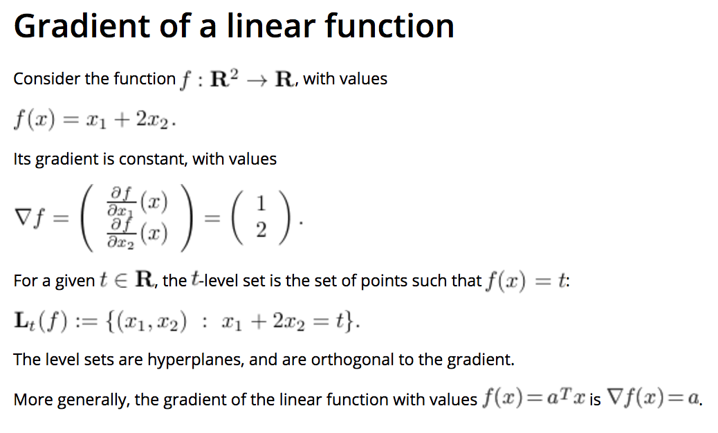
6. Gradient of a Linear Function:
   

7. Gradient of an Affine Function:

   The gradient of a function $f : \mathbf{R}^n \rightarrow \mathbf{R}$ at a point $x$, denoted $\nabla f(x)$, is the vector of first derivatives with respect to $x_1, \ldots, x_n$.

   When $n=1$ (there is only one input variable), the gradient is simply the derivative.

   An affine function $f : \mathbf{R}^n \rightarrow \mathbf{R}$, with values $f(x) = a^Tx+b$ has the gradient:

   $\nabla f(x) = a$.

   i.e. For all Affine Functions, the gradient is the constant vector $a$.

8. Interpreting $a$ and $b$:

   • The $b=f(0)$ is the constant term. For this reason, it is sometimes referred to as the bias, or intercept.

     as it is the point where $f$ intercepts the vertical axis if we were to plot the graph of the function.

   • The terms $a_j, j=1, \ldots, n,$ which correspond to the gradient of $f$, give the coefficients of influence of $x_j$ on $f$.

     For example, if $a_1 >> a_3$, then the first component of $x$ has much greater influence on the value of $f(x)$ than the third.

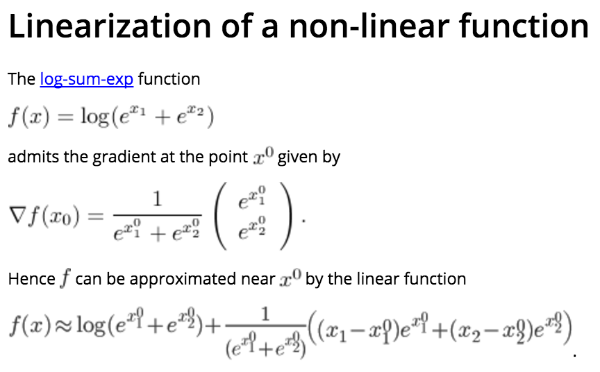
9. First-order approximation of non-linear functions:

   • One-dimensional case:
     Consider a function of one variable $f : \mathbf{R} \rightarrow \mathbf{R}$, and assume it is differentiable everywhere.
     Then we can approximate the values function at a point $x$ near a point $x_0$ as follows:

   $$f(x) \simeq l(x) := f(x_0) + f'(x_0) (x-x_0) ,$$

   $\ \ \ \ \ \ \ \\) where \(f'(x)$ denotes the derivative of $f$ at $x$.

   • Multi-dimensional:
     Let us approximate a differentiable function $f : \mathbf{R}^n \rightarrow \mathbf{R}$ by a linear function $l$, so that $f$ and $l$ coincide up and including to the first derivatives.
     The approximate function l must be of the form:

   $$l(x) = a^Tx + b,$$

   $\ \ \ \ \ \ \ \\) where \(a \in \mathbf{R}^n$ and $b \in \mathbf{R}$.

   The corresponding approximation $l$ is called the first-order approximation to $f$ at $x_0$.

   • Our condition that $l$ coincides with $f$ up and including to the first derivatives shows that we must have:

   $$\nabla l(x) = a = \nabla f(x_0), \;\; a^Tx_0 + b = f(x_0),$$

   $\ \ \ \ \ \ \ \\) where \(\nabla f(x_0)$ is the gradient, of $f$ at $x_0$.

10. First-order Expansion of a function [Theorem]:

    The first-order approximation of a differentiable function $f$ at a point $x_0$ is of the form:

    $$f(x) \approx l(x) = f(x_0) + \nabla f(x_0)^T (x-x_0)$$

    where $\nabla f(x_0) \in \mathbf{R}^n$ is the gradient of $f$ at $x_0$. Example: a linear approximation to a non-linear function.

Matrices

1. Matrix Transpose:

   $$A_{ij} = A_{ji}^T, \; \forall i, j \in \mathbf{F}$$

   • Properties:
     • $$(AB)^T = B^TA^T.$$

2. Matrix-vector product:

   $$(Ax)_i = \sum_{j=1}^n A_{ij}x_j , \;\; i=1, \ldots, m.$$

   Where the Matrix is $\in {\mathbf{R}}^{m \times n}$ and the vector is $\in {\mathbf{R}}^m$.

   Interpretations:

   1. A linear combination of the columns of $A$:
      $\ \ \ \ \ \ \ \ \ \ \ \ \ \ \ \ \ \ \ \ \ \ \ \ \ \ \ \ \ \ \ \ \ \ \ \ \ \ \ \ \ \ \ \ \ Ax = \left( \begin{array}{c} a_1^Tx \ldots a_m^Tx \end{array} \right)^T$ .
      where the columns of $A$ are given by the vectors $a_i, i=1, \ldots, n$, so that $A = (a_1 , \ldots, a_n)$.

   2. Scalar Products of Rows of $A$ with $x$:
      $\ \ \ \ \ \ \ \ \ \ \ \ \ \ \ \ \ \ \ \ \ \ \ \ \ \ \ \ \ \ \ \ \ \ \ \ \ \ \ \ \ \ \ \ \ Ax = \sum_{i=1}^n x_i a_i$ .
      where the rows of $A$ are given by the vectors $a_i^T, i=1, \ldots, m$: $A = \left( \begin{array}{c} a_1^T \ldots a_m^T \end{array} \right)^T$.

   Example: Network Flows

3. Left Product:

   If $z \in \mathbf{R}^m$, then the notation $z^TA$ is the row vector of size $n$ equal to the transpose of the column vector $A^Tz \in \mathbf{R}^n$:

   $(z^TA)_j = \sum_{i=1}^m A_{ij}z_i , \;\; j=1, \ldots, n.$ Example: Representing the constraint that the columns of a matrix sum to zero.

4. Matrix-matrix product:

   $(AB)_{ij} = \sum_{k=1}^n A_{ik} B_{kj}$.

   where $A \in \mathbf{R}^{m \times n}$ and $B \in \mathbf{R}^{n \times p}$, and the notation $AB$ denotes the $m \times p$ matrix given above.

   Interpretations:

   1. Transforming the columns of $B$ into $Ab_i$:
      $\ \ \ \ \ \ \ \ \ \ \ \ \ \ \ \ \ \ \ \ \ \ \ \ \ \ \ \ \ \ \ \ \ \ \ \ \ \ \ \ \ \ \ \ \ AB = A \left( \begin{array}{ccc} b_1 & \ldots & b_n \end{array} \right) = \left( \begin{array}{ccc} Ab_1 & \ldots & Ab_n \end{array} \right)$ .
      where the columns of $B$ are given by the vectors $b_i, i=1, \ldots, n$, so that $B = (b_1 , \ldots, b_n)$.
   2. Transforming the Rows of $A$ into $a_i^TB$:
      $\ \ \ \ \ \ \ \ \ \ \ \ \ \ \ \ \ \ \ \ \ \ \ \ \ \ \ \ \ \ \ \ \ \ \ \ \ \ \ \ \ \ \ \ \ AB = \left(\begin{array}{c} a_1^T \\ \vdots \\ a_m^T \end{array}\right) B = \left(\begin{array}{c} a_1^TB \\ \vdots \\ a_m^TB \end{array}\right)$.
      where the rows of $A$ are given by the vectors $a_i^T, i=1, \ldots, m$: $A = \left( \begin{array}{c} a_1^T \ldots a_m^T \end{array} \right)^T$.

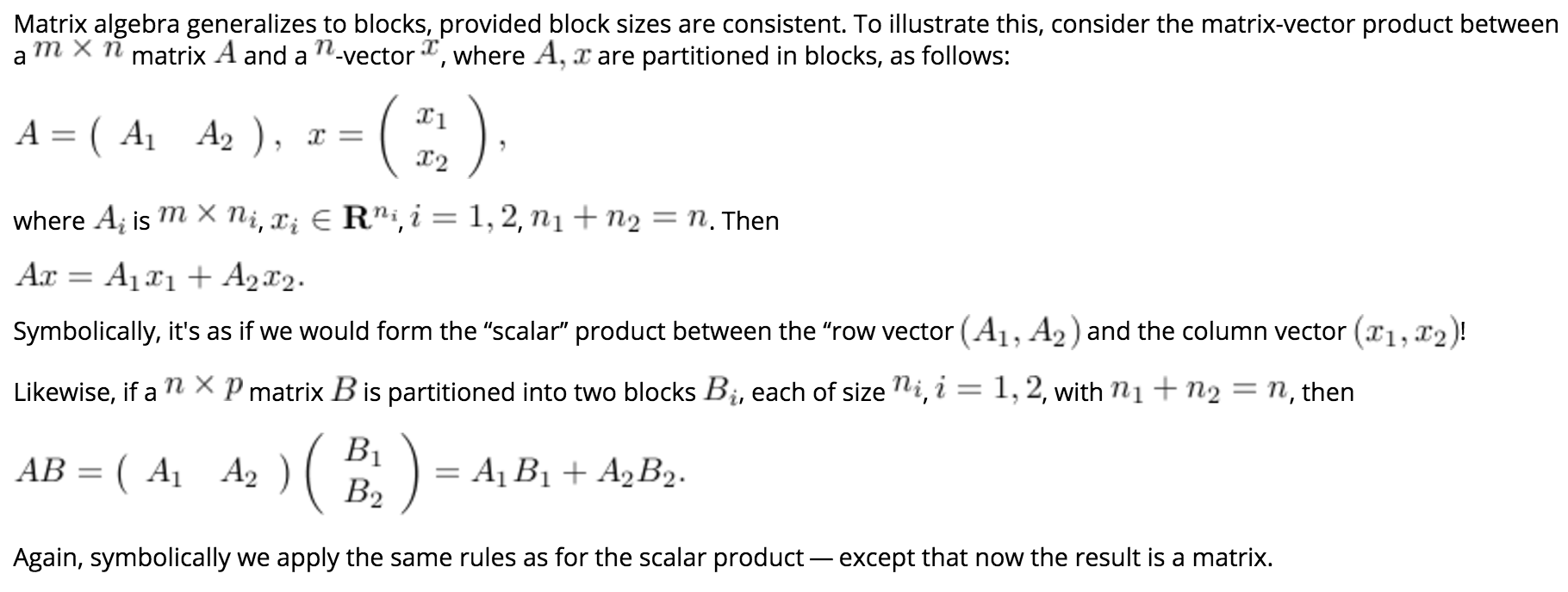
5. Block Matrix Products:
   

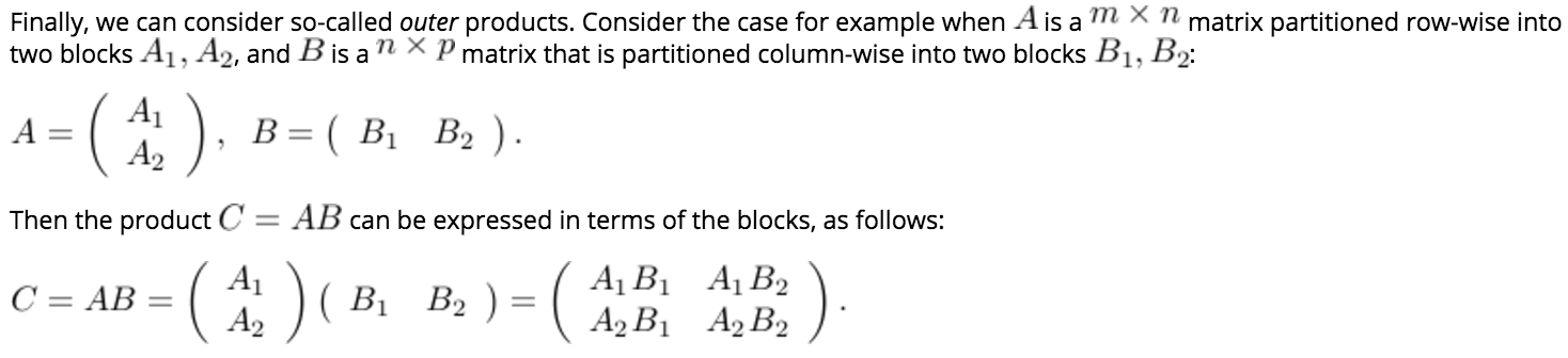
6. Outer Products:

7. Trace:

   The trace of a square $n \times n$ matrix $A$, denoted by $\mathbf{Tr} A$, is the sum of its diagonal elements:

   $\mathbf{Tr} A = \sum_{i=1}^n A_{ii}$.

   • Properties:
     • $\mathbf{Tr} A = \mathbf{Tr} A^T$.
     • $\mathbf{Tr} (AB) = \mathbf{Tr} (BA)$.
     • $\mathbf{Tr}(XYZ) = \mathbf{Tr}(ZXY) = \mathbf{Tr}(YZX)$.
     • ${\displaystyle \operatorname{tr} (A+B) = \operatorname{tr} (A)+\operatorname{tr} (B)}$.
     • ${\displaystyle \operatorname{tr} (cA) = c\operatorname{tr} (A)}$.
     • ${\displaystyle \operatorname{tr} \left(X^{\mathrm {T} }Y\right)=\operatorname{tr} \left(XY^{\mathrm {T} }\right)=\operatorname{tr} \left(Y^{\mathrm {T} }X\right)=\operatorname{tr} \left(YX^{\mathrm {T} }\right)=\sum _{i,j}X_{ij}Y_{ij}}$.
     • \({\displaystyle \operatorname{tr} \left(X^{\mathrm {T} }Y\right)=\sum _{ij}(X\circ Y)_{ij}}\ \ \ \\) (The Hadamard product).
     • Arbitrary permutations of the product of matrices is not allowed. Only, cyclic permutations are.

       However, if products of three symmetric matrices are considered, any permutation is allowed.

     • The trace of an idempotent matrix $A$, is the dimension of A.
     • The trace of a nilpotent matrix is zero.
     • If $f(x) = (x − \lambda_1)^{d_1} \cdots (x − \lambda_k)^{d_k}$ is the characteristic polynomial of a matrix $A$, then ${\displaystyle \operatorname{tr} (A)=d_{1}\lambda_{1} + \cdots + d_{k} \lambda_{k}}$.
     • When both $A$ and $B$ are $n \times n$, the trace of the (ring-theoretic) commutator of $A$ and $B$ vanishes: $\mathbf{tr}([A, B]) = 0$; one can state this as “the trace is a map of Lie algebras ${\displaystyle \mathbf{GL_{n}} \to k}$ from operators to scalars”, as the commutator of scalars is trivial (it is an abelian Lie algebra).
     • The trace of a projection matrix is the dimension of the target space. ${\displaystyle P_{X} = X\left(X^{\mathrm {T} }X\right)^{-1}X^{\mathrm {T} } \\ \Rightarrow \\ \operatorname {tr} \left(P_{X}\right) = \operatorname {rank} \left(X\right)}$

8. Scalar Product:

   $$\langle A, B \rangle := \mathbf{Tr}(A^TB) = \displaystyle\sum_{i=1}^m\sum_{j=1}^n A_{ij}B_{ij}.$$

   The above definition is Symmetric:

   $$\implies \langle A,B \rangle = \mathbf{Tr} (A^TB) = \mathbf{Tr} (A^TB)^T = \mathbf{Tr} (B^TA) = \langle B,A \rangle .$$

   We can interpret the matrix scalar product as the vector scalar product between two long vectors of length $mn$ each, obtained by stacking all the columns of $A, B$ on top of each other.

9. Special Matrices:
   
   • Diagonal matrices: are square matrices $A$ with $A_{ij} = 0$ when $i \ne j$.
   • Symmetric matrices: are square matrices that satisfy $A_{ij} = A_{ji}$for every pair $(i,j)$.

   • Triangular matrices: are square matrices that satisfy $A_{ij} = A_{ji}$for every pair $(i,j)$.
     {F}}^{2}=|AR|{\rm {F}}^{2}=|RA|{\rm {F}}^{2}}$for any rotation matrix$R$$.

     1. Invariant under a unitary transformation for complex matrices.

     2. ${\displaystyle \|A^{\rm {T}}A\|_{\rm {F}}=\|AA^{\rm {T}}\|_{\rm {F}}\leq \|A\|_{\rm {F}}^{2}}$.

     3. ${\displaystyle \|A+B\|_{\rm {F}}^{2}=\|A\|_{\rm {F}}^{2}+\|B\|_{\rm {F}}^{2}+2\langle A,B\rangle _{\mathrm {F} }}$.

10. $l_{\infty,\infty}$ (Max Norm):

    $$\|A\|_{\max} = \max_{ij} |a_{ij}|.$$

    • Properties:
      1. NOT Submultiplicative.

11. The Spectral Norm:

    ${\displaystyle \|A\|_{2}={\sqrt {\lambda _{\max }(A^{^{*}}A)}}=\sigma _{\max }(A)} = {\displaystyle \max_{\|x\|_2!=0}(\|Ax\|_2)/(\|x\|_2)}.$

    The spectral norm of a matrix ${\displaystyle A}$ is the largest singular value of ${\displaystyle A}$. i.e. the square root of the largest eigenvalue of the positive-semidefinite matrix ${\displaystyle A^{*}A}.$

    • The Spectral Radius of $A \\) [denoted \(\rho(A)$]:

      $$\lim_{r\rightarrow\infty}\|A^r\|^{1/r}=\rho(A).$$

    • Properties:

      1. Submultiplicative.

      2. Satisfies, ${\displaystyle \|A^{r}\|^{1/r}\geq \rho (A),}$, where $\rho(A)$ is the spectral radius of $A$.

      3. It is an “induced vector-norm”.

12. Asynchronous:

13. Asynchronous:

14. Equivalence of Norms:
    CLICK TO VIEW

15. Applications:
    

    1. RMS Gain: Frobenius Norm.

    2. Peak Gain: Spectral Norm.

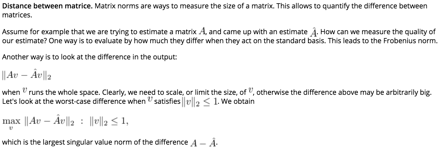
    3. Distance between Matrices: Frobenius Norm. Click to View

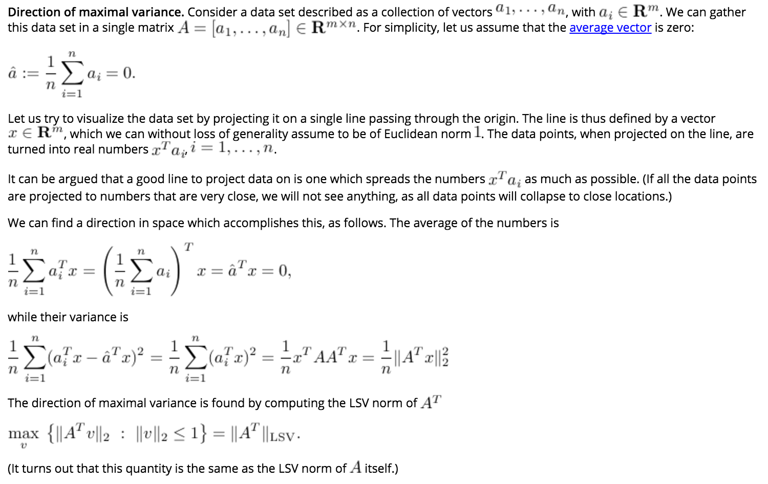
    4. Direction of Maximal Variance: Spectral Norm. Click to View