Table of Contents
Quadratic Functions
-
- What?
- A function \(q : \mathbf{R}^n \rightarrow \mathbf{R}\) is said to be a quadratic function if it can be expressed as
- \[q(x) = \sum_{i=1}^n \sum_{j=1}^n A_{ij} x_i x_j + 2 \sum_{i=1}^n b_i x_i + c,\]
- for numbers \(A_{ij}, b_i,\) and \(c, i, j \in {1, \ldots, n}\).
A quadratic function is thus an affine combination of the \(\ x_i\)’s and all the “cross-products” \(x_ix_j\).
-
We observe that the coefficient of \(x_ix_j\) is \((A_{ij} + A_{ji})\).
-
The function is said to be a quadratic form if there are no linear or constant terms in it: \(b_i = 0, c=0.\)
-
The Hessian of a quadratic function is always constant.
-
- Link between Quadratic Func’s & Symmetric Matrices:
- Indeed, any quadratic function \(q : \mathbf{R}^n \rightarrow \mathbf{R}\) can be written as
- \[q(x) = \left( \begin{array}{c} x \\ 1 \end{array} \right)^T \left( \begin{array}{cc} A & b \\ b^T & c \end{array} \right) \left( \begin{array}{c} x \\ 1 \end{array} \right) = x^TAx + 2 b^Tx + c,\]
- for an appropriate symmetric matrix \(A \in \mathbf{S}^{n}\), vector \(b \in \mathbf{R}^n\) and scalar \(c \in \mathbf{R}\).
-
\(A_{ii}\) is the coefficient of \(x_i^2\) in q;
\(2A_{ij}\) (for \(i \ne j\)) is the coefficient of the term \(x_ix_j\) in q;
\(2b_i\) is that of \(x_i\);
\(c\) is the constant term, \(q(0)\). -
If q is a quadratic form, then \(b=0, c=0,\) and we can write \(q(x) = x^TAx\) where now \(A \in \mathbf{S}^n\).
-
- Second-order approximations [1-D]:
- If \(f : \mathbf{R} \rightarrow \mathbf{R}\) is a twice-differentiable function of a single variable, then the second order approximation (or, second-order Taylor expansion) of \(f\) at a point \(x_0\) is of the form:
- \[f(x) \approx q(x) = f(x_0) + f(x_0)' (x-x_0) + \dfrac{1}{2} f''(x_0)(x-x_0)^2,\]
- where \(f'(x_0)\) is the first derivative, and f’‘(x_0) the second derivative, of \(f\) at \(x_0\).
We observe that the quadratic approximation \(q\) has the same value, derivative, and second-derivative as \(f\), at \(x_0\).
-
- Second-order approximations [n-D]:
- Let us approximate a twice-differentiable function \(f : \mathbf{R}^n \rightarrow \mathbf{R}\) by a quadratic function \(q\), so that \(f\) and \(q\) coincide up and including to the second derivatives.
- The function \(q\) must be of the form
- \[q(x) = x^TAx + 2b^Tx + c,\]
- where \(A \in \mathbf{S}^n, b \in \mathbf{R}^n\text{, and } c \in \mathbf{R}\). Our condition that q coincides with f up and including to the second derivatives shows that we must have:
- \[(1)\ \ \ \ \ \ \ \nabla^2 q(x)\ \ =\ \ 2 A =\ \ \nabla^2 f(x_0), \\ (2)\ \nabla q(x) = 2(Ax_0+b) = \nabla f(x_0), \\ (3)\ \ \ \ \ \ x_0^TAx_0 + 2b^Tx_0 + c = f(x_0). \\\]
- Solving for A,b,c we obtain the following result:
- \[f(x) \approx q(x) = f(x_0) + \nabla f(x_0)^T (x-x_0) + \dfrac{1}{2} (x-x_0)^T \nabla^2 f(x_0) (x-x_0),\]
- where \(\nabla f(x_0) \in \mathbf{R}^n\) is the gradient of \(f\) at \(x_0\), and the symmetric matrix \(\nabla^2 f(x_0)\) is the Hessian of \(f\) at \(x_0\).
Basics and Definitions
-
- Eigenvalue:
- A real scalar \(\lambda\) is said to be an eigenvalue of a matrix \(A\) if there exist a non-zero vector \(v \in \mathbf{R}^n\) such that:
- \[A v = \lambda u.\]
-
The interpretation of \(v\) is that it defines a direction along \(A\) behaves just like scalar multiplication. The amount of scaling is given by \(\lambda\).
-
- Eigenvector:
- Asynchronous: \
THIRD
- Asynchronous: \
Eigen-Stuff of Symmetric Matrices
-
- The Spectral Theorem (for Symmetric Matrices):
- We can decompose any symmetric matrix \(A \in \mathbf{S}^n\) with the symmetric eigenvalue decomposition (SED)
- \[A = \sum_{i=1}^n \lambda_i u_iu_i^T = U \Lambda U^T, \;\; \Lambda = \mathbf{diag}(\lambda_1, \ldots, \lambda_n) .\]
- where the matrix of \(U := [u_1 , \ldots, u_n]\) is orthogonal (that is, \(U^TU=UU^T = I_n\)), and contains the eigenvectors of \(A\), while the diagonal matrix Lambda contains the eigenvalues of \(A\).
The SED provides a decomposition of the matrix in simple terms, namely dyads.

-
- Spectral Decomposition:
- \[Au_j = \sum_{i=1}^n \lambda_i u_iu_i^Tu_j = \lambda_j u_j, \;\; j=1, \ldots, n.\]
-
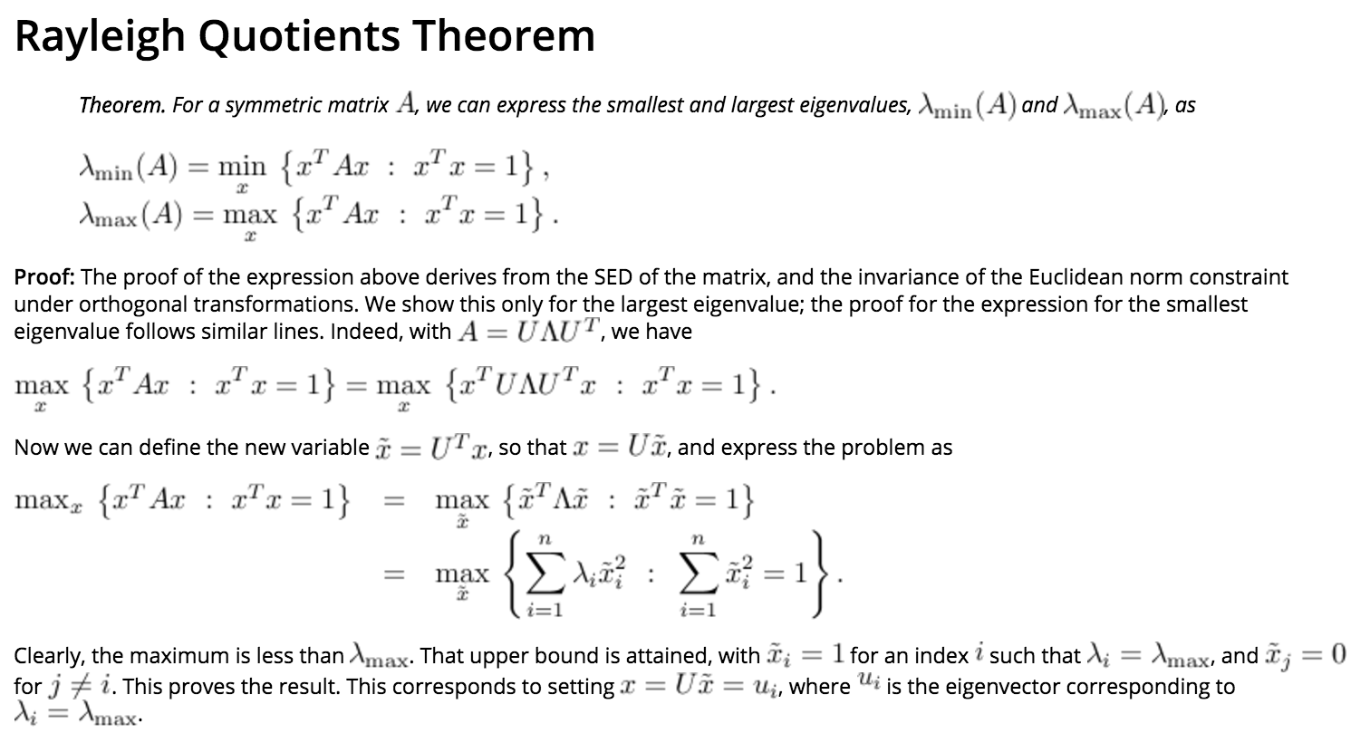
- Rayleigh Quotients:
- Given a symmetric matrix \(A\), we can express the smallest and largest eigenvalues of \(A\), denoted \(\lambda_{\rm min}\) and \(\lambda_{\rm max}\) respectively, in the so-called variational form:
- \[\lambda_{\rm min}(A) = \min_{x} : \left\{ x^TAx ~:~ x^Tx = 1 \right\} , \\ \lambda_{\rm max}(A) = \max_{x} : \left\{ x^TAx ~:~ x^Tx = 1 \right\} .\]
-
The term “variational” refers to the fact that the eigenvalues are given as optimal values of optimization problems, which were referred to in the past as variational problems.
Variational representations exist for all the eigenvalues, but are more complicated to state. -

-
- Interptation:
The interpretation of the above identities is that the largest and smallest eigenvalues is a measure of the range of the quadratic function \(x \rightarrow x^TAx\) over the unit Euclidean ball.
The quantities above can be written as the minimum and maximum of the so-called Rayleigh quotient \(\dfrac{x^TAx}{x^Tx}\).
- Interptation:
-
Example: Largest singular value norm of a matrix
Visit the Book
- Asynchronous:
Positive Definitness
-
- Associated Quadratic Form:
- For a given symmetric matrix \(A \in \mathbf{R}^{n \times n}\), the associated quadratic form is the function \(q : \mathbf{R}^n \rightarrow \mathbf{R}\) with values: \(q(x) = x^TAx.\)
-
- Positive Definite Matrices:
- A symmetric matrix \(A\) is said to be positive definite (PD, notation: \(A \succ 0\)) if and only if the associated quadratic form \(q\) is positive everywhere:
- \[q(x) > 0 \mbox{ for every } x \in \mathbf{R}^n.\]
-
- Positive Semi-Definite Matrices:
- A symmetric matrix \(A\) is said to be positive semi-definite (PSD, notation: \(A \succeq 0\)) if and only if the associated quadratic form \(q\) is non-negative everywhere:
- \[q(x) \ge 0 \mbox{ for every } x \in \mathbf{R}^n.\]
-
- Definite Matrices:
- When \(q = 0\).
-
- Diagonal Matrices and Positive Definitness:
-
Diagonal matrices. A diagonal matrix is PSD (resp. PD) if and only if all of its (diagonal) elements are non-negative (resp. positive).
-
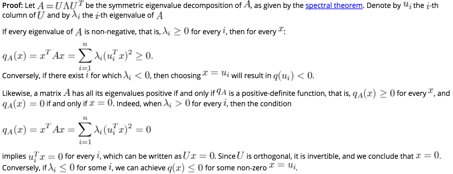
- Theorem. Spectral Decomposition of PSD Matrices:
- A quadratic form \(q(x) = x^TAx\), with \(A \in \mathbf{S}^n\) is non-negative (resp. positive-definite) if and only if every eigenvalue of the symmetric matrix A is non-negative (resp. positive).

-
- Square Roots of PSD Matrices:
- If A is PSD, there exist a unique PSD matrix, denoted \(A^{1/2}\), such that \(A = (A^{1/2})^2\).
- We can express this matrix square root in terms of the SED of \(A = U\Lambda U^T,\) as \(A^{1/2} = U \Lambda^{1/2} U^T\), where \(\Lambda^{1/2}\) is obtained from \(\Lambda\) by taking the square root of its diagonal elements.
- If \(A\) is PD, then so is its square root.
-
- The Cholesky Decomposition: \
- Any PSD matrix can be written as a product \(A = LL^T\) for an appropriate matrix \(L\).
- The decomposition is not unique, and \(L = A^{1/2}\) is only a possible choice (the only PSD one).
- Another choice, in terms of the SED of \(A = U^T \Lambda U\), is \(L = U^T \Lambda^{1/2}\).
- If \(A\) is positive-definite, then we can choose \(L\) to be lower triangular, and invertible. The decomposition is then known as the Cholesky decomposition of \(A\).
-
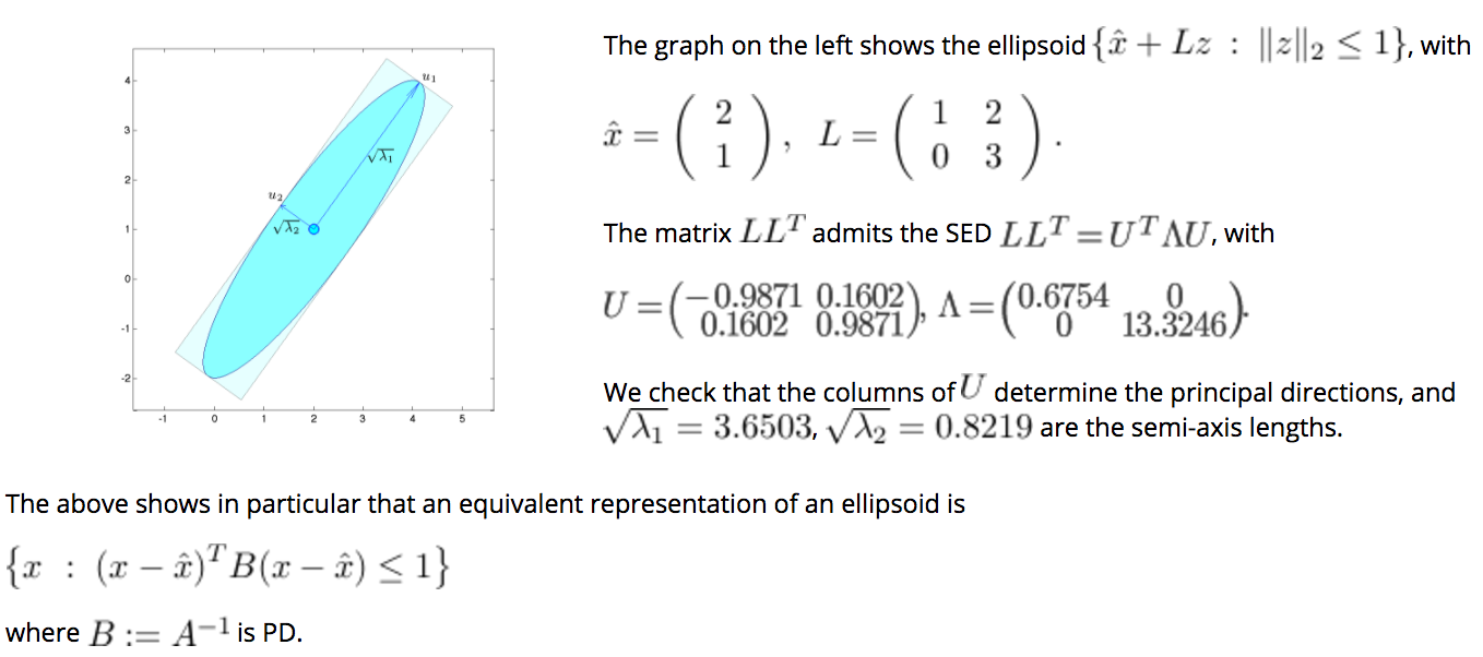
- Ellipsoids and PSDs:
- Definition. We define an ellipsoid to be affine transformation of the unit ball for the Euclidean norm:
- \[\mathbf{E} = \left\{ \hat{x} + L z ~:~ \|z\|_2 \le 1 \right\} ,\]
- where \(L \in \mathbf{R}^{n \times n}\) is an arbitrary non-singular (invertible) matrix.
- We can express the ellipsoid as:
- \[\mathbf{E} = \left\{ x ~:~ \|L^{-1}(x-\hat{x})\|_2 \le 1 \right\} = \left\{ x ~:~ (x-\hat{x})^T A^{-1} (x-\hat{x}) \le 1 \right\} ,\]
- where \(A=LL^T\) is PD.
-
- Geometric Interpretation via SED:
- We interpret the eigenvectors and associated eigenvalues of A in terms of geometrical properties of the ellipsoid, as follows.
- Consider the SED of \(A: A = U \Lambda U^T\), with \(U^TU = I\) and \(\Lambda\) diagonal, with diagonal elements positive.
- The SED of its inverse is \(A^{-1} = L L^T = U \Lambda^{-1} U^T\).
- Let \(\tilde{x} = U^T(x-\hat{x})\).
- We can express the condition \(x \in \mathbf{E}\) as:
- \[\tilde{x}^T\Lambda^{-1}\tilde{x} = \displaystyle\sum_{i=1}^n \frac{\tilde{x}_i^2}{\lambda_i} \le 1.\]
-
- Now set \(\bar{x}_i := \tilde{x}_i/\sqrt{\lambda_i} , i=1, \ldots, n\).
- The above writes \(\bar{x}^T\bar{x} \le 1: \in \bar{x}-\)space, the ellipsoid is simply an unit ball.
- In \(\tilde{x}-\)space, the ellipsoid corresponds to scaling each \(\bar{x}-\)axis by the square roots of the eigenvalues.
- The ellipsoid has principal axes parallel to the coordinate axes in \(\tilde{x}-\)space.
- We then apply a rotation and a translation, to get the ellipsoid in the original x-space.
- The rotation is determined by the eigenvectors of \(A^{-1}\), which are contained in the orthogonal matrix \(U\).
- Thus, the geometry of the ellipsoid can be read from the SED of the PD matrix \(A^{-1} = LL^T \\ \implies\)
(1) The eigenvectors give the principal directions, and
(2) The semi-axis lengths are the square root of the eigenvalues.
-

-
It is possible to define degenerate ellipsoids, which correspond to cases when the matrix B in the above, or its inverse A, is degenerate. For example, cylinders or slabs (intersection of two parallel half-spaces) are degenerate ellipsoids.