The Singular Value Decomposition
-
- What?
- Recall from here that any matrix \(A \in \mathbf{R}^{m \times n}\) with rank one can be written as \(A = \sigma u v^T\), where \(u \in \mathbf{R}^m, v \in \mathbf{R}^n,\) and \(\sigma >0.\)
- It turns out that a similar result holds for matrices of arbitrary rank \(r\). : That is, we can express any matrix \(A \in \mathbf{R}^{m \times n}\) as sum of rank-one matrices:
- \[A = \sum_{i=1}^r \sigma_i u_i v_i^T,\]
- where \(u_1, \ldots, u_r\) are mutually orthogonal, \(v_1, \ldots, v_r\) are also mutually orthogonal, and the \(\sigma_i\)’s are positive numbers called the singular values of \(A\).
-
- The SVD Theorem:
- An arbitrary matrix \(A \in \mathbf{R}^{m \times n}\) admits a decomposition of the form:
- \[A = \sum_{i=1}^r \sigma_i u_i v_i^T = U \tilde{ {S}} V^T, \;\; \tilde{ {S}} := \left( \begin{array}{cc} {S} & 0 \\ 0 & 0 \end{array} \right) ,\]
- where \(U \in \mathbf{R}^{m \times m}, V \in \mathbf{R}^{n \times n}\) are both orthogonal matrices, and the matrix \(S\) is diagonal:
- \[S = \mathbf{diag}(\sigma_1 , \ldots, \sigma_r),\]
- where,
- The positive numbers \(\sigma_1 \ge \ldots \ge \sigma_r > 0\) are unique, and are called the singular values of A.
- The number \(r \le min(m,n)\) is equal to the rank of \(A\).
- The triplet \((U, \tilde{ {S}}, V)\) is called a singular value decomposition (SVD) of \(A\).
- The first \(r\) columns of \(U: u_i, i=1, \ldots, r\) (resp. \(V: v_i, i=1, \ldots, r)\) are called left (resp. right) singular vectors of \(A\), and satisfy:
- \[Av_i = \sigma_i u_i, \;\;\;\; A^Tu_i = \sigma_i v_i, \;\;\;\; i=1,...,r.\]
-

Notes:
- \(\begin{array}{l}{U^{T} U=I} \\ {V^{T} V=I}\end{array}\) are orthogonal matrices with orthonormal eigenvector basis
- If \(\boldsymbol{v}\) is eigenvector of \(X^TX\) then \(X\boldsymbol{v}\) is eigenvector of \(XX^T\)
-
- Computing the SVD:
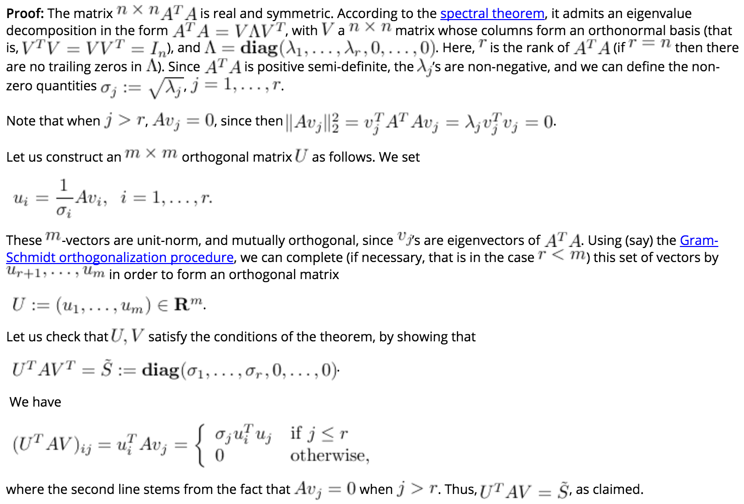
- To find the SVD of a matrix \(A\), we solve the following equation:
- \[\begin{align} & (1)\ A^TA = V\Lambda^T\Lambda V^T \\ & (2)\ AV\ = U \Lambda \end{align}\]
- Complexity of the SVD:
- Normal Matrices: the complexity grows as \(\mathcal{O}(nm \: min(n,m))\).
- Sparse Matrices: good approximations can be calculated very efficiently.
-
- Geometric Interpretation:
- The theorem allows to decompose the action of A on a given input vector as a sequence of three elementary transformations.
- First, we form \(\tilde{x} := V^Tx \in \mathbf{R}^n\).
\(V\) orthogonal \(\implies \tilde{x}\) is a rotated version of \(x\), which still lies in the input space.
- Then we act on the rotated vector \(\tilde{x}\) by scaling its elements
The first \(k\) elements of \(\tilde{x}\) are scaled by the singular values \(\sigma_1, \ldots, \sigma_r\); the remaining \(n-r\) elements are set to zero.
This step results in a new vector \(\tilde{y}\) which now belongs to the output space \(\mathbf{R}^m\). - Finally, we rotate the vector \(\tilde{y}\) by the orthogonal matrix \(U\), which results in \(y = U\tilde{y} = Ax\).
Notice also: \(\tilde{x} : = V^Tx, \ x = V\tilde{x}.\)
- First, we form \(\tilde{x} := V^Tx \in \mathbf{R}^n\).
- Summary:
- A rotation in the input space
- A scaling that goes from the input space to the output space
- A rotation in the output space.
In contrast with symmetric matrices, input and output directions are different.
-

-
- Link with the Spectral Theorem:
- If \(A\) admits an SVD, then the matrices \(AA^T\) and \(A^TA\) has the following SEDs:
- \[AA^T = U \Lambda_m U^T, \;\; A^TA = V \Lambda_n V^T,\]
- where \(\Lambda_m := \tilde{ {S}}\tilde{ {S}}^T = \mathbf{ diag}(\sigma_1^2, \ldots, \sigma_r^2, 0, \ldots, 0)\) is \(m \times m\) (so it has \(m-r\) trailing zeros),
and \(\Lambda_n := \tilde{ {S}}^T\tilde{ {S}} = \mathbf{ diag}(\sigma_1^2, \ldots, \sigma_r^2, 0, \ldots, 0)\) is \(n \times n\) (so it has \(n-r\) trailing zeros). -
The eigenvalues of \(AA^T\) and \(A^TA\) are the same, and equal to the squared singular values of \(A\).
The corresponding eigenvectors are the left and right singular vectors of \(A\).
Matrix Properties via SVD
-
- Nullspace:
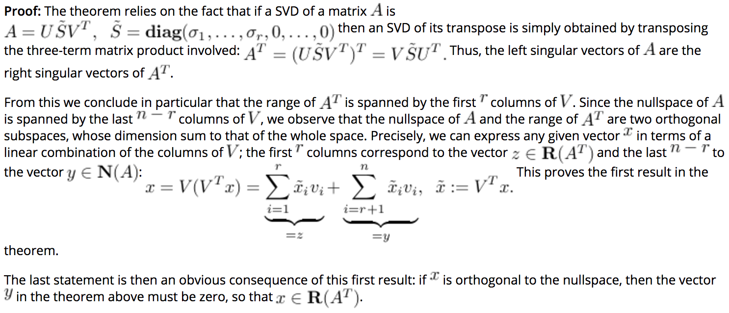
- The SVD allows to compute an orthonormal basis for the nullspace of a matrix.
-
- Theorem: Nullspace via SVD:
- The nullspace of a matrix A with SVD
- \[A = U \tilde{S} V^T, \;\; \tilde{S} := \left( \begin{array}{cc}S & 0 \\ 0 & 0 \end{array} \right) , \;\; S = \mathbf{diag}(\sigma_1 , \ldots, \sigma_r),\]
- where \(U \in \mathbf{R}^{m \times m}, V \in \mathbf{R}^{n \times n}\) are both orthogonal matrices, admits the last \(n-r\) columns of \(V\) as an orthonormal basis.
-
- Full Column-Rank Matrices:
- ne-to-one (or, full column rank) matrices are the matrices with nullspace reduced to {0}. If the dimension of the nullspace is zero, then we must have n=r. Thus, full column rank matrices are ones with SVD of the form
- \[A = U \left( \begin{array}{c} {S} \\ 0 \end{array} \right) V^T.\]
-
- Theorem: Range and Rank via SVD:
- The range of a matrix \(A\) with SVD
- \[A = U \tilde{ {S}} V^T, \;\; \tilde{ {S}} = \mathbf{diag}(\sigma_1, \ldots, \sigma_r, 0, \ldots, 0)\]
- where \(U \in \mathbf{R}^{m \times m}, V \in \mathbf{R}^{n \times n}\) are both orthogonal matrices, admits the first \(r\) columns of \(U\) as an orthonormal basis.
-
- Full Row Rank Matrices.:
- An onto (or, full row rank) matrix has a range \(r=m\).
These matrices are characterized by an SVD of the form - \[A = U \left( \begin{array}{cc} {S} & 0 \end{array} \right) V^T.\]
-
- Fundamental theorem of linear algebra:
- Let \(A \in \mathbf{R}^{m \times n}\). The sets \(\mathbf{N} (A)\) and \(\mathbf{R} (A^T)\) form an orthogonal decomposition of \(\mathbf{R}^n\), in the sense that any vector \(x \in \mathbf{R}^n\) can be written as
- \[x = y + z, \;\; y \in \mathbf{N} (A), \;\; z \in \mathbf{R} (A^T), \;\; y^Tz = 0.\]
- In particular, we obtain that the condition on a vector \(x\) to be orthogonal to any vector in the nullspace implies that it must be in the range:
- \[x^Ty = 0 \mbox{ whenever } Ay = 0 \Longleftrightarrow \exists \: \lambda \in \mathbf{R}^m ~:~ x = A^T\lambda.\]
-

-
- Matrix Norms:
- Matrix norms, which are useful to measure the size of a matrix, can be interpreted in terms of input-output properties of the corresponding linear map; for example, the Frobenius norm measure the average response to unit vectors, while the largest singular (LSV) norm measures the peak gain.
These two norms can be easily read from the SVD. -
- Frobenius Norm:
- \[\|A\|_F = \sqrt{\mathbf{Tr} A^TA}\]
- \(\:\:\:\:\:\:\:\:\:\) Using the SVD \((U, \tilde{ {S}}, V)\) of \(A\), we obtain
-
\[\|A\|_F^2 = \mathbf{Tr} (V \tilde{ {S}}^T \tilde{ {S}} V^T) = \mathbf{Tr} (V^TV \tilde{ {S}}^T \tilde{ {S}}) = \mathbf{Tr} (\tilde{ {S}}^T \tilde{ {S}}) = \sum_{i=1}^r \sigma_i^2.\]
Hence the squared Frobenius norm is nothing else than the sum of the squares of the singular values.
-
- Largest Singular Value Norm.: measures a matrix size based on asking the maximum ratio of the norm of the output to the norm of the input. When the norm used is the Euclidean norm, the corresponding quantity
- \[\|A\|_{\rm LSV} := \max_x : \|Ax\|_2 ~:~ \|x\|_2 \le 1 = \max_{x \:\:\: \|x\|_2 \le 1} : \|Ax\|_2 = \sigma_1(A),\]
- \(\:\:\:\:\:\:\:\:\:\) where \(\sigma_1(A)\) is the largest singular value of \(A\), is called the largest singular value (LSV) norm.
Any left singular vector associated with the largest singular value achieves the maximum in the above.
-
- Condition Number:
- The condition number of an invertible n times n matrix A is the ratio between the largest and the smallest singular values:
- \(\kappa(A) = \frac{\sigma_1}{\sigma_n} = \|A\| \cdot \|A^{-1}\|.\)
Provides a measure of the sensitivity of the solution of a linear equation to changes in \(A\).