Point-Set Topology

1. Open Set:

   A set \(\chi \subseteq \mathbf{R}^n\) is said to be open if for any point \(x \in \chi\) there exist a ball centered in \(x\) which is contained in \(\chi\).

   Precisely, for any \(x \in \mathbf{R}^n\) and \(\epsilon > 0\) define the Euclidean ball of radius \(r\) centered at \(x\):

   \[B_\epsilon(x) = {z : \|z − x\|_2 < \epsilon}\]

   Then, \(\chi \subseteq \mathbf{R}^n\) is open if

   \[\forall x \: \epsilon \: \chi, \:\: \exists \epsilon > 0 : B_\epsilon(x) \subset \chi .\]

   Equivalently,

   • A set \(\chi \subseteq \mathbf{R}^n\) is open if and only if \(\chi = int\; \chi\).

   • An open set does not contain any of its boundary points.

   • A closed set contains all of its boundary points.

   • Unions and intersections of open (resp. closed) sets are open (resp. closed).

2. Closed Set:

   A set \(\chi \subseteq \mathbf{R}^n\) is said to be closed if its complement \(\mathbf{R}^n \text{ \ } \chi\) is open.

3. Interior of a Set:

   The interior of a set \(\chi \subseteq \mathbf{R}^n\) is defined as

   \[int\: \chi = \{z \in \chi : B_\epsilon(z) \subseteq \chi, \:\: \text{for some } \epsilon > 0 \}\]

4. Closure of a Set:

   The closure of a set \(\chi \subseteq \mathbf{R}^n\) is defined as

   \[\bar{\chi} = \{z ∈ \mathbf{R}^n : \: z = \lim_{k\to\infty} x_k, \: x_k \in \chi , \: \forall k\},\]

   i.e., the closure of \(\chi\) is the set of limits of sequences in \(\chi\).

5. Boundary of a Set:

   The boundary of X is defined as

   \[\partial \chi = \bar{\chi} \text{ \ } int\: \chi\]

6. Bounded Set:

   A set \(\chi \subseteq \mathbf{R}^n\) is said to be bounded if it is contained in a ball of finite radius, that is if there exist \(x \in \mathbf{R}^n\) and \(r > 0\) such that \(\chi \subseteq B_r(x)\).

7. Compact Set:

   A set \(\chi \subseteq \mathbf{R}^n\) is compact \(\iff\) it is Closed and Bounded.

8. Relative Interior [\(\operatorname{relint}\)]:

   We define the relative interior of the set \(\chi\), denoted \(\operatorname{relint} \chi\), as its interior relative to \(\operatorname{aff} C\):

   \[\operatorname{relint} \chi = \{x \in \chi : \: B(x, r) \cap \operatorname{aff} \chi \subseteq \chi \text{ for some } r > 0\},\]

   where \(B(x, r) = \{y : ky − xk \leq r\}\), the ball of radius \(r\) and center \(x\) in the norm \(\| · \|\).

9. Relative Boundary:

   We can then define the relative boundary of a set \(\chi\) as \(\mathbf{cl} \chi \text{ \ } \operatorname{relint} \chi,\) where \(\mathbf{cl} \chi\) is the closure of \(\chi\).

Sets Combinations and Hulls

1. Lines and Line Segments [Linear Sets]:

   Suppose \(x_1 \ne x_2\) are two points in \(\mathbf{R}^n\)

   Points of the form,

   \(y = \theta x_1 + (1 − \theta)x_2\),

   where, \(\theta \in \mathbf{R}\), form the line passing through \(x_1\) and \(x_2\).

   The parameter value \(\theta = 0\) corresponds to \(y = x_2\), and the parameter value \(\theta = 1\) corresponds to \(y = x_1\).

   Values of the parameter \(\theta\) between 0 and 1 correspond to the (closed) line segment between \(x_1\) and \(x_2\).

2. Affine Sets:

   An affine set is a translation of a subspace — it is “flat” but does not necessarily pass through 0, as a subspace would.

   (Think for example of a line, or a plane, that does not go through the origin.)

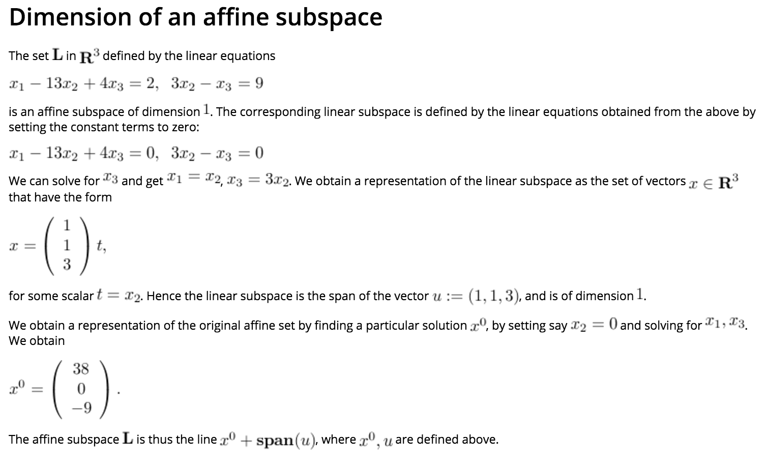
   An affine set \(\mathbf{A}\) can always be represented as the translation of the subspace spanned by some vectors:

   \(\mathbf{A} = \left\{ x_0 + \sum_{i=1}^m \lambda_i x_i ~:~ \lambda \in {\mathbf{R}}^m \right\}\ \ \\), for some vectors \(x_0, x_1, \ldots, x_m.\)

   \[\implies \mathbf{A} = x_0 + \mathbf{S}.\]

   • (Special case) lines: When \(\mathbf{S}\) is the span of a single non-zero vector, the set \(\mathbf{A}\) is called a line passing through the point \(x_0\). Thus, lines have the form \(\left\{ x_0 + tu ~:~ t \in \mathbf{R} \right\}\),
     where \(u\) determines the direction of the line, and \(x_0\) is a point through which it passes.

   • Example: Diminsion of Affine Subspaces

3. Cones [Cone Sets]:

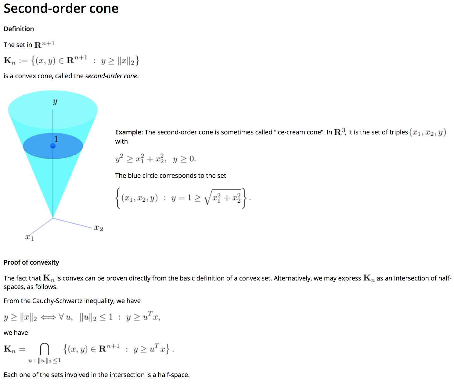
   A set \(C\) is a cone if \(x \in C\), then \(\alpha x \in C\), for every \(\alpha \geq 0\).

   A set C is said to be a convex cone if it is convex and it is a cone.

   The conic hull of a set is a convex cone.

4. Linear Combination:

   A Linear Combination is an expression constructed from a set of terms by multiplying each term by a constant and adding the results.

   \[\sum_{i=1}^n \lambda_i x_i\]

5. Affine Combination:

   An Affine Combination of the points is a special type of linear combination, in which the coefficients \(\lambda_i\) are restricted to sum up to one, that is

   \[\sum_{i=1}^n \lambda_i x_i \: : \:\: \sum_{i=1}^m \lambda_i = 1\]

   Intuitively, a convex combination is a weighted average of the points, with weights given by the \(\lambda_i\) coefficients.

6. Conical Combination:

   A Conical Combination of the points is a special type of linear combination, in which the coefficients \(\lambda_i\) are restricted to be nonnegative, that is:

   \[\sum_{i=1}^n \lambda_i x_i \: : \:\: \lambda_i \geq 0 \: \text{for all } i\]

7. Convex Combination:

   A Convex Combination of the points is a special type of linear combination, in which the coefficients \(\lambda_i\) are restricted to be nonnegative and to sum up to one, that is

   \[\lambda_i \geq 0 \: \text{for all } i, \: \text{ and } \sum_{i=1}^m \lambda_i = 1\]

   Intuitively, a convex combination is a weighted average of the points, with weights given by the \(\lambda_i\) coefficients.

8. Linear Hull:

   Given a set of points (vectors) \(\in \mathbf{R}^n:\)

   \[P = \{x^{(1)} , . . . , x^{(m)} \},\]

   The linear hull (subspace) generated by these points is the set of all possible linear combinations of the points:

   \[x=\lambda_1x^{(1)} + \cdots + \lambda_mx^{(m)}, \:\: \text{for } \lambda_i \in \mathbf{R}, \: i \in \{1, \cdots, m\}\]

9. Affine Hull:

   The affine hull, \(\operatorname{aff}\: P\), of \(P\) is the set generated by taking all possible linear combinations of the points in \(P\), under the restriction that the coefficients \(\lambda_i\) sum up to one, that is \(\sum_{i=1}^m \lambda_i = 1\).

   \(\operatorname{aff}\: P\) is the smallest affine set containing \(P\).

   • Props.
     • It is the smallest affine set containing \(\chi\).
     • or, The intersection of all affine sets containing \(\chi\).
     • \[{\displaystyle \mathrm {aff} (\mathrm {aff} (S))=\mathrm {aff} (S)}\]
     • \({\mathrm{aff}}(S)\) is a closed set
     • \[{\displaystyle \mathrm {aff} (S+F)=\mathrm {aff} (S)+\mathrm {aff} (F)}\]
     • Affine Hull is bigger than or equal to the convex hull.
     • The linear span of \(\chi\) contains the affine hull of \(\chi\).

   • Examples:
     • The affine hull of a singleton (a set made of one single element) is the singleton itself.
     • The affine hull of a set of two different points is the line through them.
     • The affine hull of a set of three points not on one line is the plane going through them.
     • The affine hull of a set of four points not in a plane in \(\mathbf{R}^3\) is the entire space \(\mathbf{R}^3\).

10. Convex Hull:

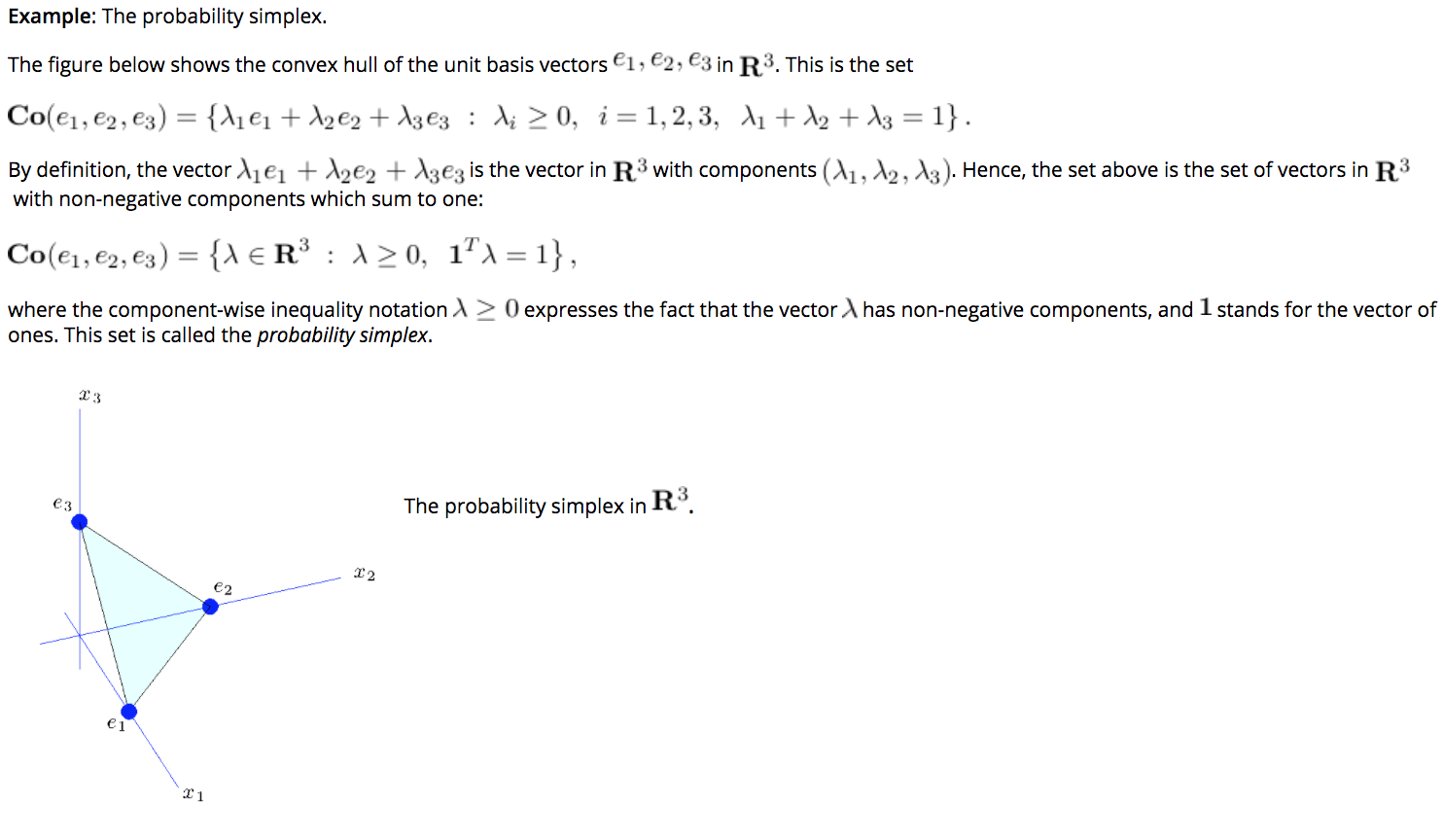
    The set of all possible convex combination is called the convex hull of the point set \(\chi\) in the Euclidean plane or in a Euclidean space (or, more generally, in an affine space over the reals) is the smallest convex set that contains \(\chi\):

    \[\mathbf{conv} (x^{(1)}, \cdots, x^{(m)}) = \left\{\sum_{i=1}^m \lambda_i x^{(i)} : \: \lambda_i \geq 0, \: i \in \{1, \cdots, m\}; \:\: \sum_{i=1}^m \lambda_i = 1\right\}\]

    • Props.
      • The convex hull of the given points is identical to the set of all their convex combinations.
      • It is the intersection of all convex sets containing \(\chi\).
      • or, The set of all convex combinations of points in \(\chi\).
      • or, The (unique) minimal convex set containing \(\chi\).
      • or, The union of all simplices with vertices in \(\chi\).
      • The algorithmic problem of finding the convex hull of a finite set of points in the plane or other low-dimensional Euclidean spaces is one of the fundamental problems of computational geometry.
      • The convex hull of a finite point set \({\displaystyle S\subsetneq \mathbb {R} ^{n}}\) forms a convex polygon when \(n = 2\),
      • or more generally a convex polytope in \({\displaystyle \mathbb {R} ^{n}}\).

11. Conic Hull:

    The set of all possible conical combinations is called the conic hull of the point set:

    \[\mathbf{conic} (x^{(1)}, \cdots, x^{(m)}) = \left\{\sum_{i=1}^m \lambda_i x^{(i)} : \: \lambda_i \geq 0, \: i \in \{1, \cdots, m\} \right\}\]

    • Props.
      • The conical hull of a set \(\chi\) is a convex set.
      • In fact, it is the intersection of all convex cones containing \(\chi\) plus the origin.
      • If \(\chi\) is a compact set (in particular, when it is a finite non-empty set of points), then the condition “plus the origin” is unnecessary.
      • If we discard the origin, we can divide all coefficients by their sum to see that a conical combination is a convex combination scaled by a positive factor.
      • Conical combinations and hulls may be considered as convex combinations and convex hulls in the projective space.
      • The conic hull of a closed set is not, even, necessarily a closed set.
      • While the convex hull of a compact set is a compact set as well, this is not so for the conical hull: the latter is Unboudned.

Convex Set

1. Convex Set:

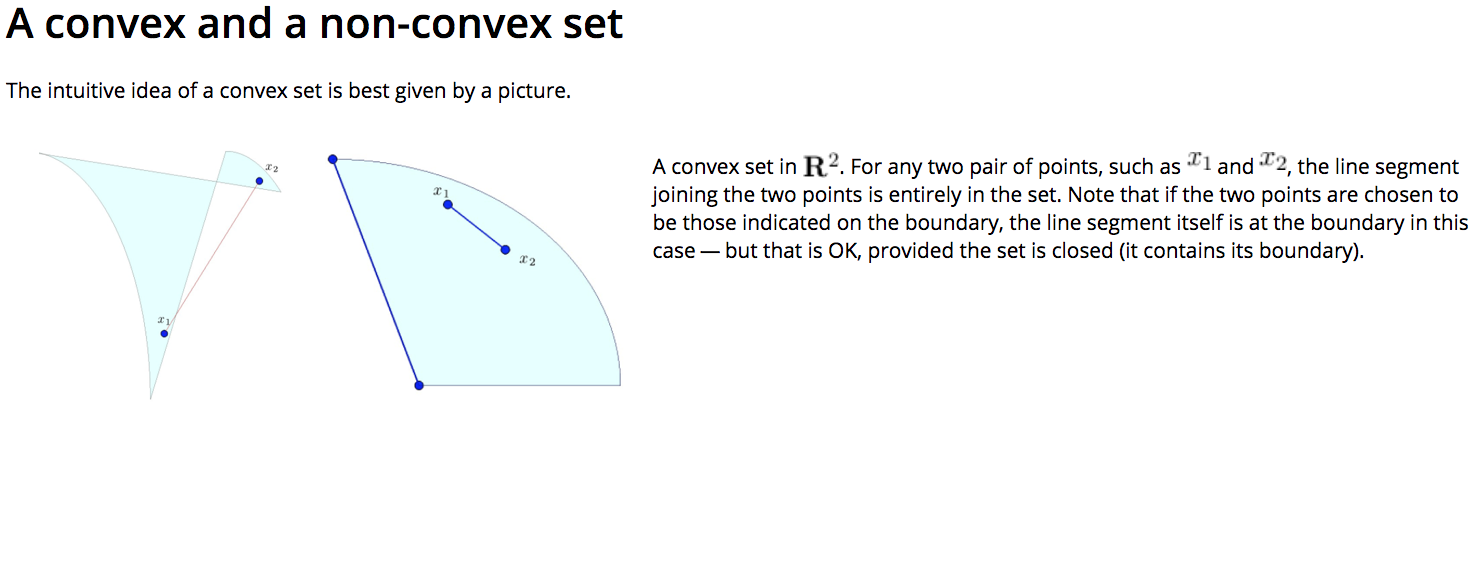
   A subset \(\mathbf{C}\) of \(\mathbf{R}^n\) is said to be convex if and only if it contains the line segment between any two points in it:

   \[\forall : x_1, x_2 \in \mathbf{C}, \;\; \forall : \lambda \in [0,1] \::\: \lambda x_1 + (1-\lambda) x_2 \in \mathbf{C}\]

2. Strictly Convex Set:

   A set C is said to be strictly convex if it is convex, and

   \[x_1 \ne x_2 \in C, \: \lambda \in (0, 1) \implies \lambda x_1 + (1 − \lambda)x_2 \in \mathbf{relint} C\]

3. Strongly Convex:

   A function \(f: \mathbf{R}^n \rightarrow \mathbf{R}\) is strongly convex if there exist a \(m > 0\) such that \(\tilde{f}(x) = f(x) − \dfrac{m}{2}\|x\|_2^2\) is convex, that is if

   \[f(\theta x + (1-\theta) y) \leq \theta f(x) + (1-\theta) f(y) - \dfrac{m}{2}\theta(1-\theta) \|x-y\|_2^2\]

4. Diminsion:

   The dimension d of a convex set \(C \subseteq \mathbf{R}^n\) is defined as the dimension of its affine hull.

   It can happen that \(d < n\).

   e.g., \(C = \left\{x = \left[\alpha 0\right]^T : \; \alpha ∈ [0, 1]\right\}\) is a convex subset of \(\mathbf{R}^2\) , with affine dimension \(d = 1\).

Prominant Examples

1. Convex Examples:

   Subspaces and affine sets, such as lines and hyperplanes are obviously convex, as they contain the entire line passing through any two points.

   Half-spaces are also convex.

   • Convex and Non-Convex Sets

   • The probability simplex

2. Asynchronous: \

3. Asynchronous: \

4. Asynchronous: \

Operators and Convexity

1. Intersection:

   The intersection of a (possibly infinite) family of convex sets is convex. This property can be used to prove convexity for a wide variety of situations.

   Ex: An halfspace \(H = \{x \in \mathbf{R}^n : \: c^Tx \leq d\}, c \ne 0\) is a convex set. The intersection of \(m\) halfspaces \(H_i, i = 1, \cdots, m\), is a convex set called a polyhedron.

   • Second-order Cone

   • Semi-definite Cone

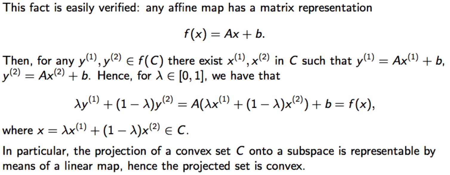
2. Affine Transformation:

   If a map \(f \: \mathbf{R}^n \rightarrow \mathbf{R}^m\) is affine, and \(\mathbf{C}\) is convex, then the set

   \[f(\mathbf{C}) \: = \left\{ f(x) : \: x \in \mathbf{C} \right\}\]

   is convex.

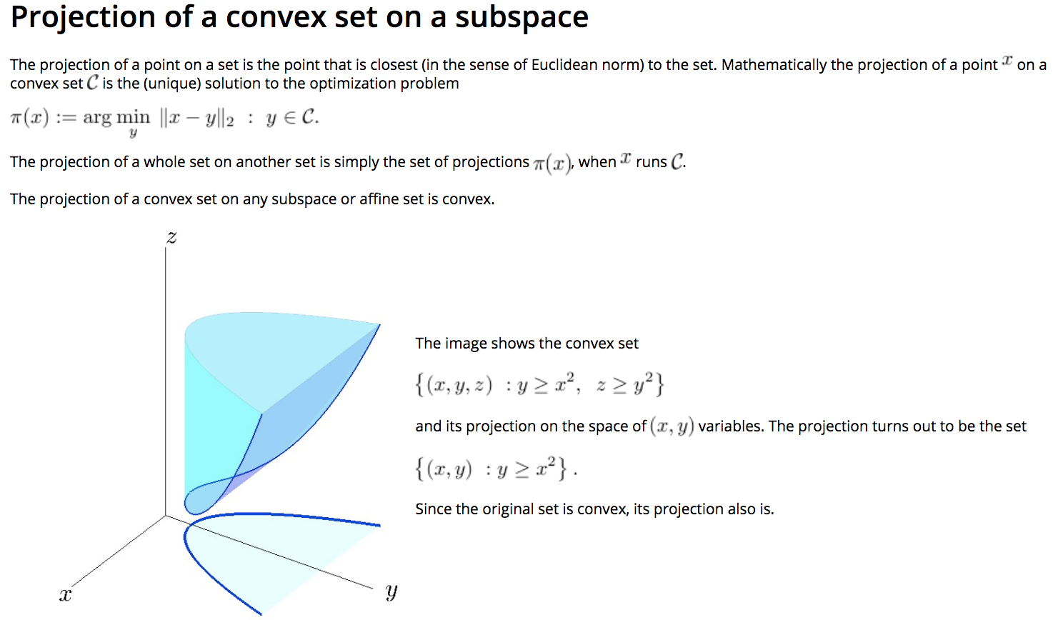
   In particular, the projection of a convex set on a subspace is convex.

   Proof.

   Example: Projection of a convex set on a subspace.

3. Composition w/ Affine Function:

   The composition with an affine function preserves convexity:

   If \(A \in \mathbf{R}^{m \times n}, b \in \mathbf{R}^m \text{ and } f : \mathbf{R}^m \rightarrow \mathbf{R}\)

   is convex, then the function \(g : \mathbf{R}^n \rightarrow \mathbf{R}\) with values \(g(x) = f(Ax+b)\) is convex.

4. Point-Wise Maximum:

   The pointwise maximum of a family of convex functions is convex:

   If \((f_\alpha)_{\alpha \in {\cal A}}\) is a family of convex functions index by \(\alpha\), then the function

   \[f(x) := \max_{\alpha \in {\cal A}} : f_\alpha(x)\]

   is convex.

   Proof.

   Ex. Convexity of the Dual Norm

   Ex. Convexity of the Largest Singular Value Function

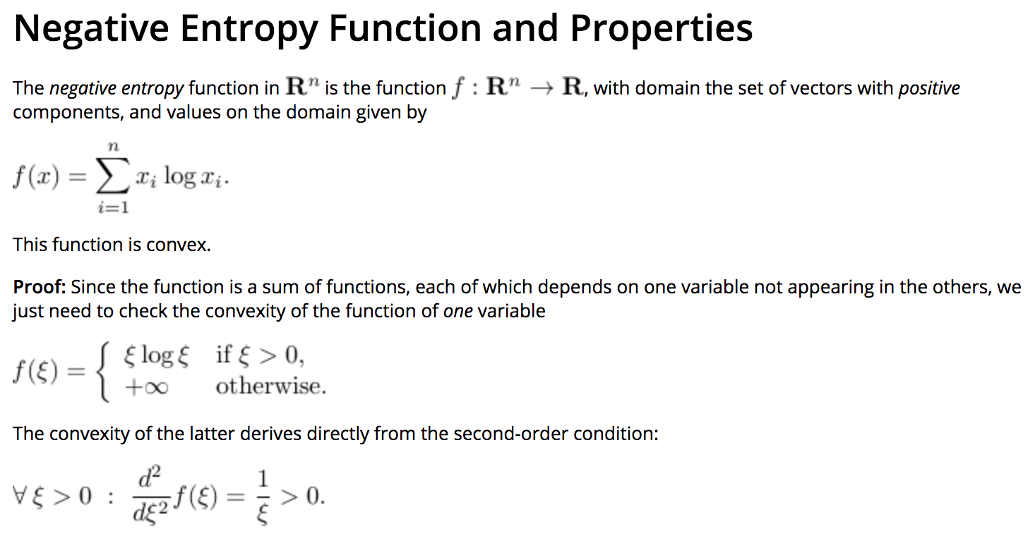
5. Nonnegative Weighted Sum:

   The nonnegative weighted sum of convex functions is convex.

   Ex. Convexity of the Negative Entropy Function

   Proof.

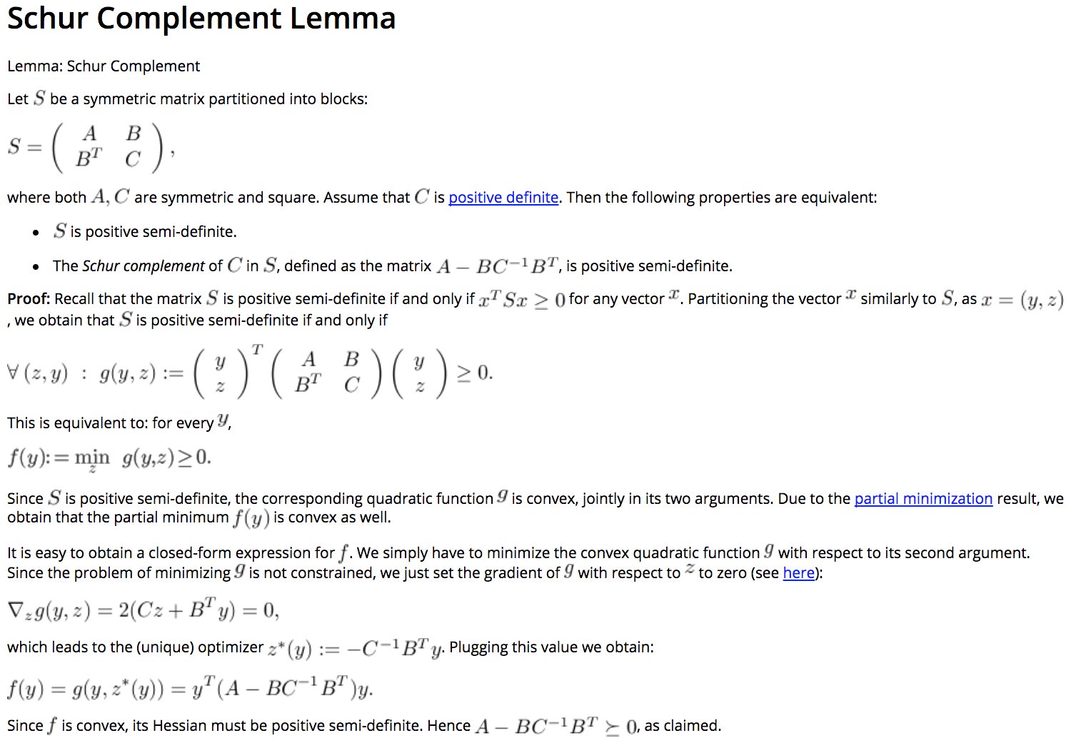
6. Partial Minimum:

   If \(f\) is a convex function in \(x=(y,z),\) then the function

   \[g(y) := \min_z \: f(y,z)\]

   is convex.

   Note that joint convexity in \((y,z)\) is essential.

   Ex. Schurs Complement Lemma

7. Composition W/ Monotone Convex Functions.:

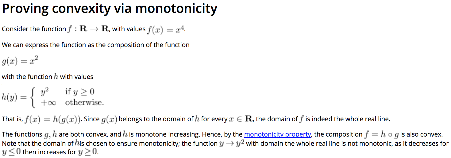
   The composition with another function does not always preserve convexity. However, if f = h circ g, with h,g convex and h increasing, then f is convex.

   Indeed, the condition \(f(x) \le t\) is equivalent to the existence of \(y\) such that

   \[h(y) \le t, \;\; g(x) \le y\]

   The condition above defines a convex set in the space of \((x,y,t)\)-variables.

   The epigraph of \(f\) is thus the projection of that convex set on the space of \((x,t)\)-variables, hence it is convex.

   Ex. Convexity via Monotonicity.

• Further Analysis:

  More generally, if the functions \(g_i : \mathbf{R}^n \rightarrow \mathbf{R}, i=1, \ldots, k\) are convex and \(h : \mathbf{R}^k \rightarrow \mathbf{R}\) is convex and non-decreasing in each argument, with \(\mathbf{dom}g_i = \mathbf{dom} h = \mathbf{R}\), then

  \[x \rightarrow (h \circ g)(x) \: = h(g_1(x), \ldots, g_k(x))\]

  is convex.

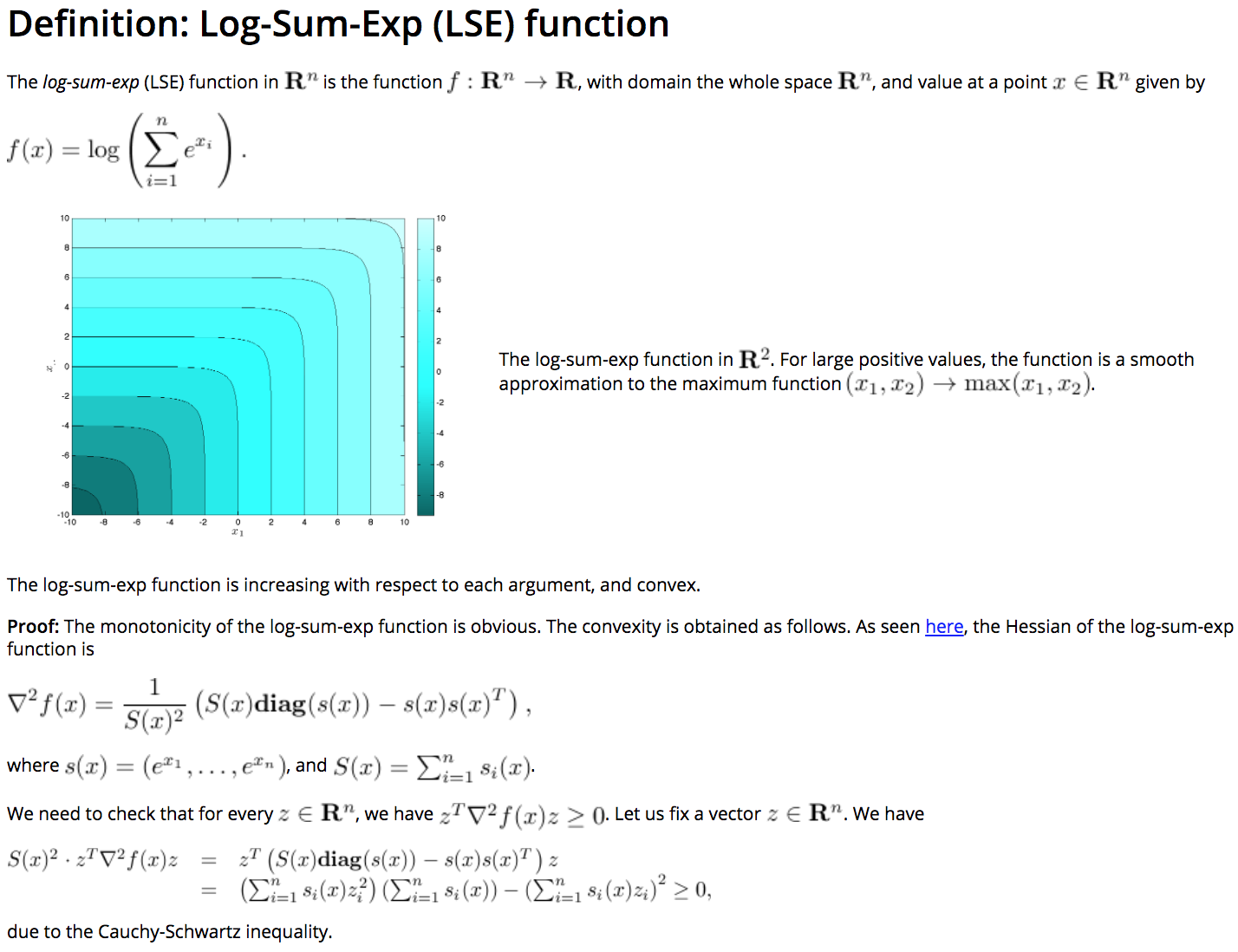
  For example, if \(g_i\)’s are convex, then \(log \sum_i \exp{g_i}\) also is.

Seperation Theorems

Separation theorems are one of the most important tools in convex optimization. They convey the intuitive idea that two convex sets that do not intersect can be separated by a straight line.

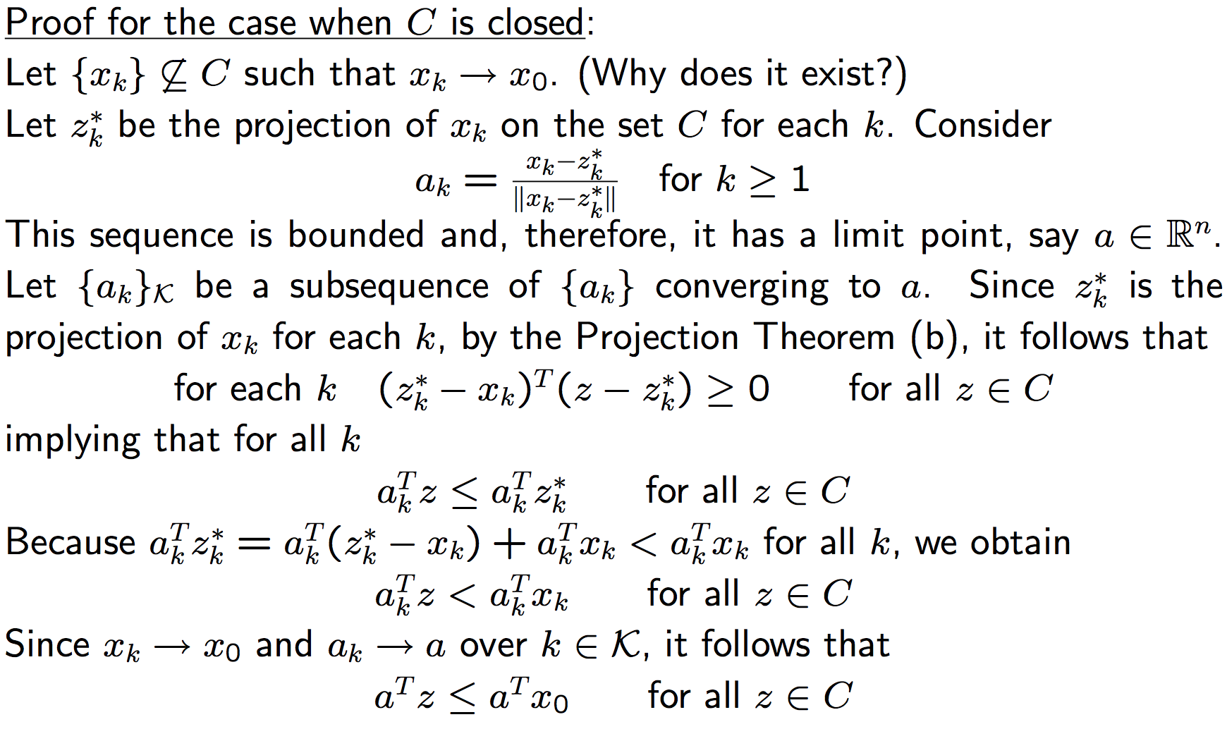
1. Theorem. Supporting Hyperplane:

   If \(\mathbf{C} \subseteq \mathbf{R}^n\) is convex and non-empty, then for any \(x_0\) at the boundary of \(\mathbf{C}\), there exist a supporting hyperplane to \(\mathbf{C}\) at \(x_0\),
   meaning that there exist \(a \in \mathbf{R}^n, \: a \ne 0,\) such that \(a^T(x-x_0) \le 0\) for every \(x \in \mathbf{C}\).

   Proof.

2. Theorem. Separating Hyperplane:

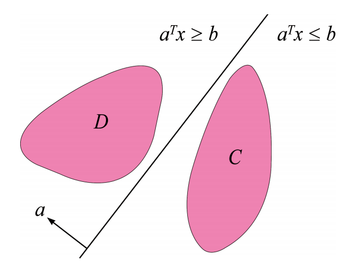
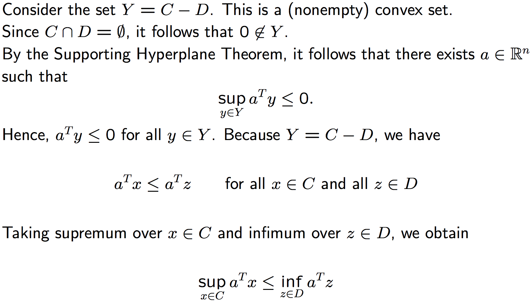
   If \(\mathbf{C}, \mathbf{D}\) are two convex subsets of \(\mathbf{R}^n\) that do not intersect, then there is an hyperplane that separates them,
   that is, \(\exists a \in \mathbf{R}^n, \: a \ne 0,\) and \(b \in \mathbf{R}\), such that \(a^Tx \le b\) for every \(x \in \mathbf{C}\), and \(a^Tx \ge b\) for every \(x \in \mathbf{D}\).

   Equivalently,

   Let C, D ⊆ Rn be nonempty convex disjoint sets i.e., \(C \cap D = \varnothing\).

   Then, there exists a hyperplane separating these sets, i.e.,

   \(\exists a \in \mathbf{R}^n, \: a \ne 0\), such that

   \[\sup_{x\in C} a^Tx \: \leq \: \sup_{z\in D}a^Tz\]

   

   Proof.

   When two convex sets do not intersect, it is possible to find a hyperplane that separates them.

3. Theorem. Strictly Separating Hyperplane:

   Let \(C, D \subseteq \mathbf{R}^n\) be nonempty convex disjoint sets.

   Assume that \(C − D\) is closed. Then, there exists a hyperplane strictly. separating the sets, i.e., \(\exists \: a \in \mathbf{R}^n, \: a \ne 0,\) such that

   \[\sup_{x\in C} a^Tx \: < \: \sup_{z\in D}a^Tz\]

   When is \((C − D)\) closed?

   One of conditions: \(C\) is closed and \(D\) is compact.

4. Farkas lemma:

   Let \(A \in \mathbf{R}^{m \times n}\) and \(y \in \mathbf{R}^m\). Then, one and only one of the following two conditions is satisfied:

   1. The system of linear equations \(Ax = y\) admits a nonnegative solution \(x \geq 0\).
   2. There exist \(z \in \mathbf{R}^m\) such that \(z^TA \geq 0, \: z^Ty < 0\).

   • Equivalent Formulation: statement (2) above implies the negation of statement (1), and vice versa. Thus, the following two statements are equivalent:
     1. There exist \(x \geq 0\) such that \(Ax = y\).
     2. \(z^Ty \geq 0, \:\: \forall z : \: z^TA \geq 0\).

   • Interpretation in terms of systems of linear inequalities: Let \(a_i \in \mathbf{R}^m, i = 1, \cdots, n\), be the columns of \(A\), then

   \[y^Tz \geq 0, \forall z : a_i^Tz \geq 0, i = 1, \cdots, n\]

   if and only if there exist multipliers \(x_i \geq 0, i = 1, \cdots, n\) such that \(y\) is a conic combination of the \(a_i\)’s:

   \[\exists x_i \geq 0, i = 1, \cdots, m : \: y = a_1x_1 + \cdots + a_nx_n.\]

Convex Functions

1. Domain:

   The domain of a function \(f: \mathbf{R}^n \rightarrow \mathbf{R}\) is the set \(\mathbf{dom} f \subseteq \mathbf{R}^n\) over which \(f\) is well-defined, in other words:

   \[\mathbf{dom} f \: = \{ x \in \mathbf{R}^n : \: -\infty < f(x) < +\infty\}.\]

2. Convex Function:

   A function \(f : \mathbf{R}^n \rightarrow \mathbf{R}\) is convex if

   (1) Its domain \(\mathbf{dom} f\) is convex.

   (2) And, \(\forall \:\: x, y \in \mathbf{dom} f , \;\; \forall \theta \in [0,1] : \:\: f(\theta x + (1-\theta) y) \le \theta f(x) + (1-\theta) f(y).\)

   Note that the convexity of the domain is required.

3. Concave Function:

   A function \(f\) is concave if the function \(-f\) is convex.

4. Convexity and the Epigraph:

   A function \(f : \mathbf{R}^n \rightarrow \mathbf{R}\), is convex if and only if, its epigraph,

   \[\mathbf{ epi } f \:= \: \left\{ (x,t) \in \mathbf{R}^{n+1} : \: t \ge f(x) \right\}\]

   is convex.

   Example: We can us this result to prove for example, that the largest eigenvalue function \(\lambda_{\rm max} : \mathcal{S}^n \rightarrow \mathbf{R}\), which to a given \(n \times n\) symmetric matrix \(X\) associates its largest eigenvalue, is convex, since the condition \(\lambda_{\rm max}(X) \le t\) is equivalent to the condition that \(t I - X \in \mathcal{S}_+^n\).

5. First-order condition:

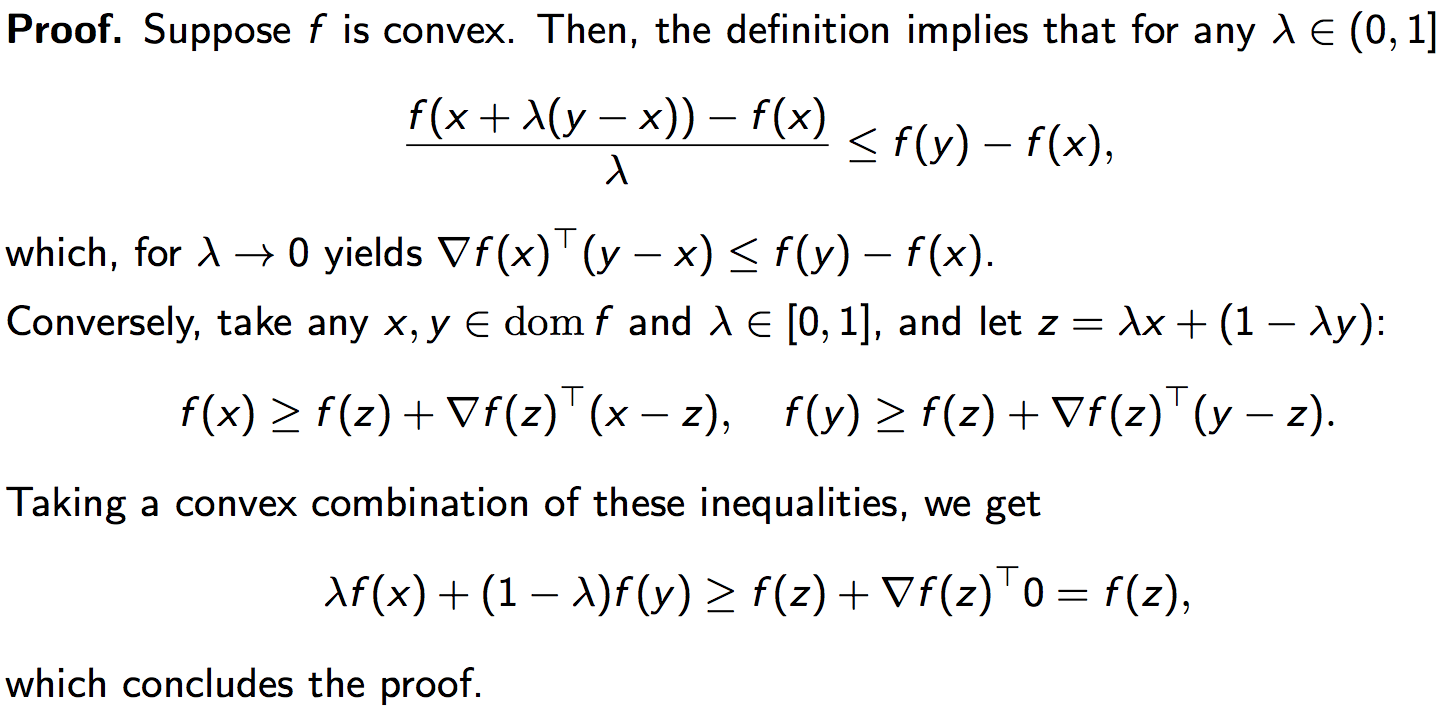
   If f is differentiable (that is, \(\mathbf{dom} f\) is open and the gradient exists everywhere on the domain), then \(f\) is convex if and only if

   \[\forall : x, y : \: f(y) \ge f(x) + \nabla f(x)^T(y-x) .\]

   The geometric interpretation is that the graph of \(f\) is bounded below everywhere by anyone of its tangents.

   Convexity of the log-sum-exp function.

   

6. Restriction to a line:

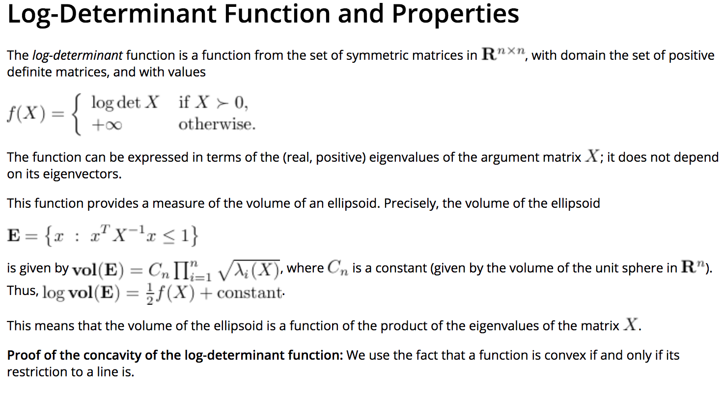
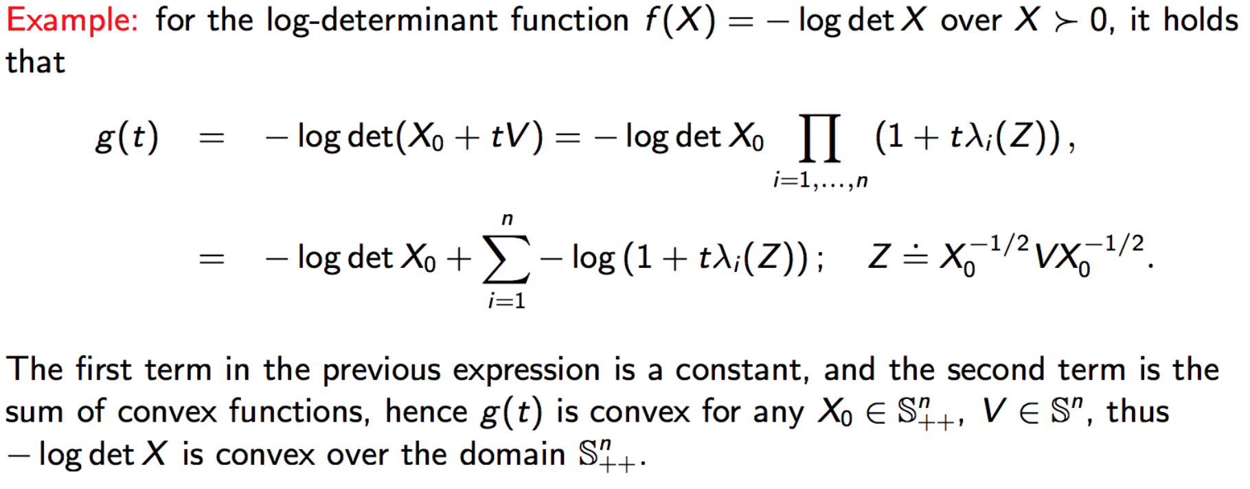
   The function \(f\) is convex if and only if its restriction to any line is convex, meaning that

   for every \(x_0 \in \mathbf{R}^n\), and \(v \in \mathbf{R}^n\), the function \(g(t) := f(x_0+tv)\) is convex.

   Note that the “if” part is a direct consequence of the “composition with an affine function” result below.

   Example: Diminsion of Affine Subspaces

   Example: sum log

7. Second-order Condition:

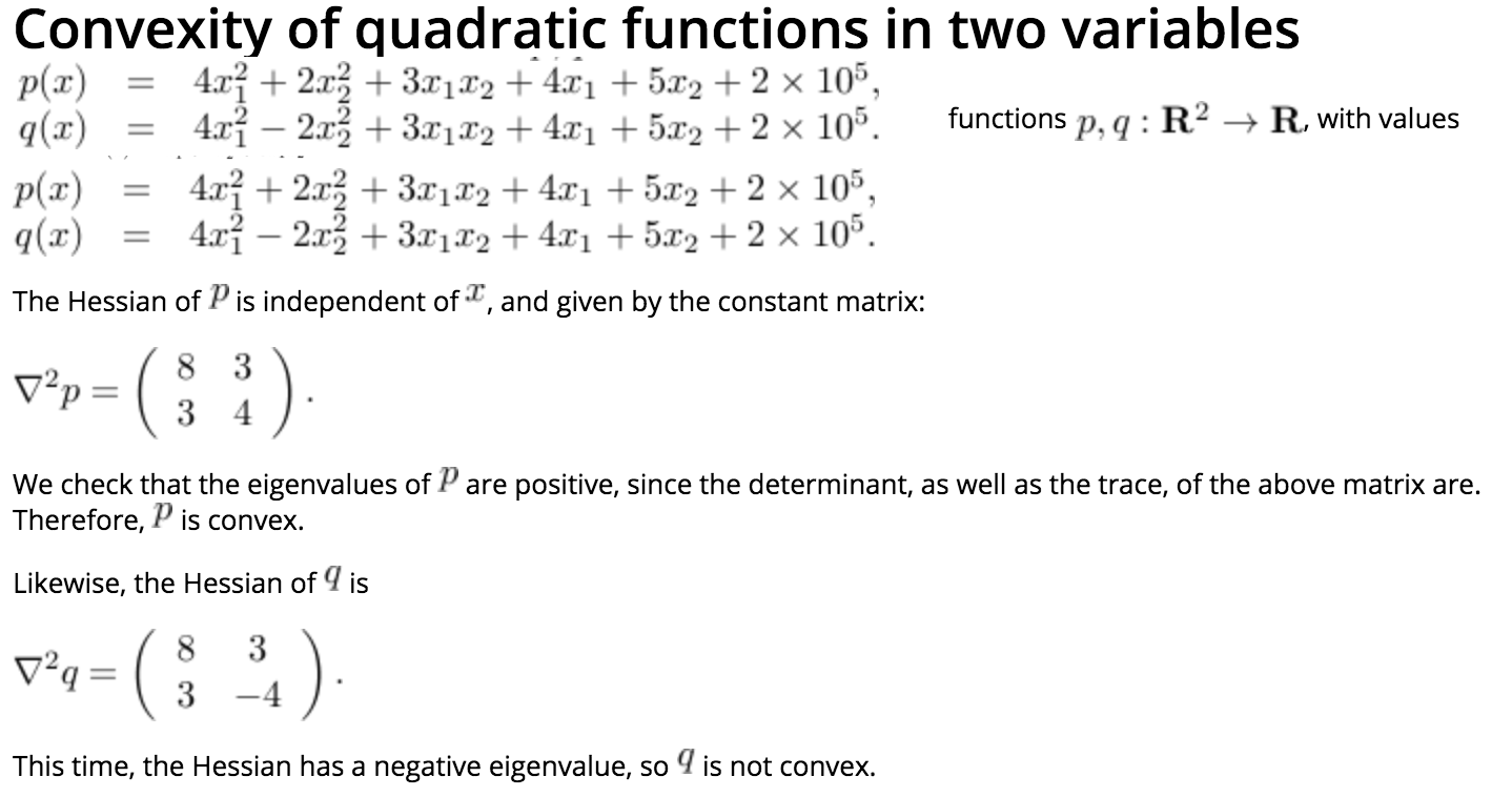
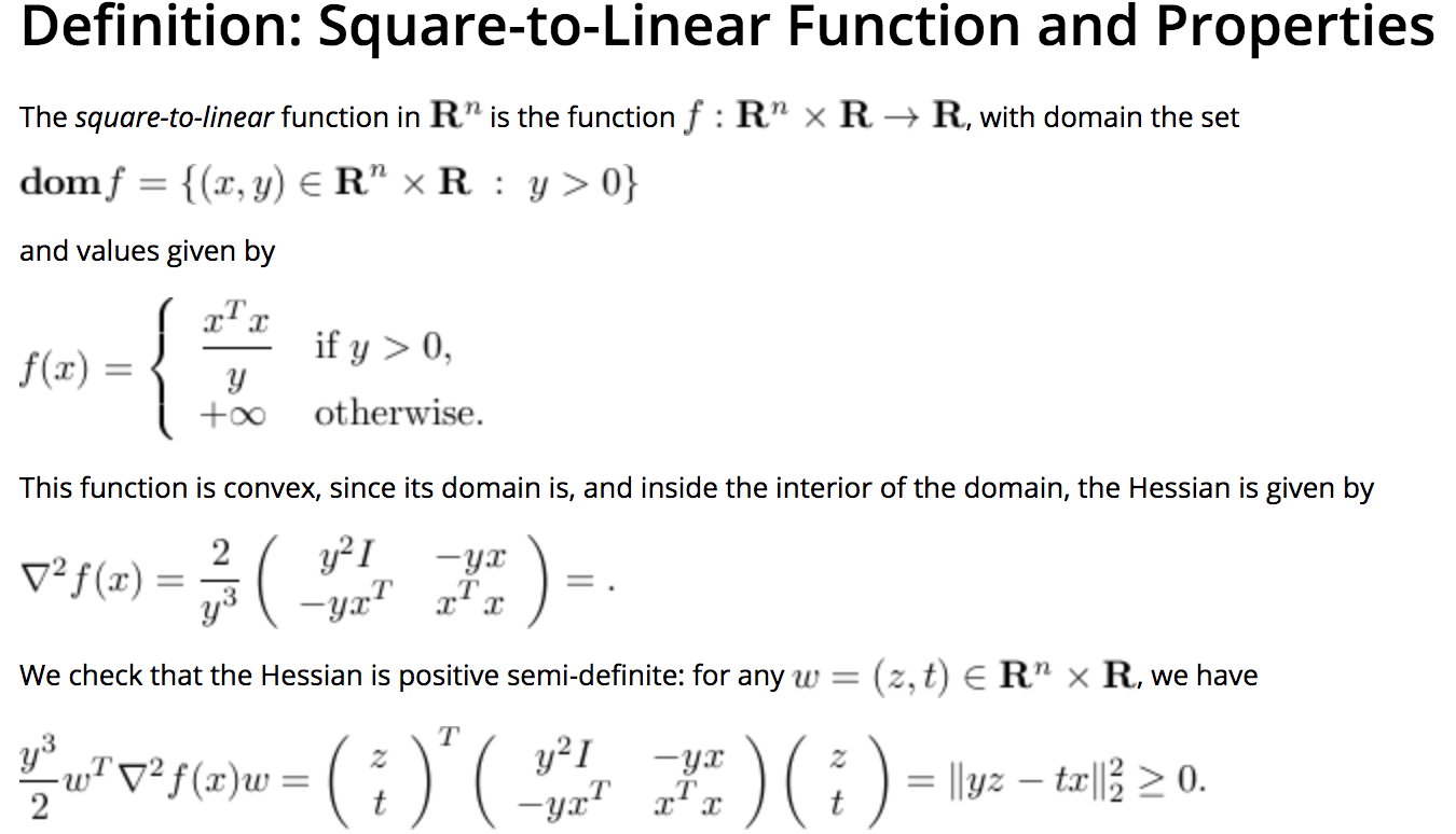
   If \(f\) is twice differentiable, then it is convex if and only if its Hessian \(\nabla^2 f\) is positive semi-definite everywhere on the domain of \(f\).

   This is perhaps the most commonly known characterization of convexity.

   Also, If \(f\) is twice differentiable, then it is Strictly convex if and only if its Hessian \(\nabla^2 f\) is positive definite everywhere on the domain of \(f\).

   Finally, If \(f\) is twice differentiable, then it is Strongly convex if and only if its Hessian \(\nabla^2 f \succeq ml\), for some \(m > 0\) and for all \(x \in \mathbf{dom} f\).

   Convexity of a quadratic function.

   Convexity of the square-to-linear function

   Convexity of the log-sum-exp function.

   Example.