Resources:

• VAEs (pdf)
• Scalable semi-supervised learning with deep variational autoencoders (Code)
• Tutorial: Categorical Variational Autoencoders using Gumbel-Softmax (+Code)
• Variational Autoencoders Pursue PCA Directions [by Accident] (paper!)
• Latent Variable Models and AutoEncoders (Intuition Blog!)
• Tutorial: Categorical Variational Autoencoders using Gumbel-Softmax (Kingma)

Variational Auto-Encoders

Auto-Encoders (click to read more) are unsupervised learning methods that aim to learn a representation (encoding) for a set of data in a smaller dimension.
Auto-Encoders generate Features that capture factors of variation in the training data.

1. Auto-Regressive Models VS Variational Auto-Encoders:

   Auto-Regressive Models defined a tractable (discrete) density function and, then, optimized the likelihood of training data:

   \[p_\theta(x) = p(x_0) \prod_1^n p(x_i | x_{i<})\]

   On the other hand, VAEs defines an intractable (continuous) density function with latent variable \(z\):

   \[p_\theta(x) = \int p_\theta(z) p_\theta(x|z) dz\]

   but cannot optimize directly; instead, derive and optimiz a lower bound on likelihood instead.

2. Variational Auto-Encoders (VAEs):

   Variational Autoencoder models inherit the autoencoder architecture, but make strong assumptions concerning the distribution of latent variables.

   They use variational approach for latent representation learning, which results in an additional loss component and specific training algorithm called Stochastic Gradient Variational Bayes (SGVB).

3. Assumptions:

   VAEs assume that:

   • The data is generated by a directed graphical model \(p(x\vert z)\)
   • The encoder is learning an approximation \(q_\phi(z|x)\) to the posterior distribution \(p_\theta(z|x)\)
     where \({\displaystyle \mathbf {\phi } }\) and \({\displaystyle \mathbf {\theta } }\) denote the parameters of the encoder (recognition model) and decoder (generative model) respectively.
   • The training data \(\left\{x^{(i)}\right\}_{i=1}^N\) is generated from underlying unobserved (latent) representation \(\mathbf{z}\)

4. The Objective Function:

   $${\displaystyle {\mathcal {L}}(\mathbf {\phi } ,\mathbf {\theta } ,\mathbf {x} )=D_{KL}(q_{\phi }(\mathbf {z} |\mathbf {x} )||p_{\theta }(\mathbf {z} ))-\mathbb {E} _{q_{\phi }(\mathbf {z} |\mathbf {x} )}{\big (}\log p_{\theta }(\mathbf {x} |\mathbf {z} ){\big )}}$$

   where \({\displaystyle D_{KL}}\) is the Kullback–Leibler divergence (KL-Div).

   Notes:

   • \(\boldsymbol{z}\) is some latent vector (representation); where each element is capturing how much of some factor of variation that we have in our training data.
     e.g. attributes, orientations, position of certain objects, etc.

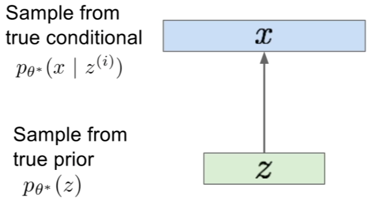
5. The Generation Process:
   

6. The Goal:
   The goal is to estimate the true parameters \(\theta^\ast\) of this generative model.
   
   

7. Representing the Model:
   - To represent the prior \(p(z)\), we choose it to be simple, usually Gaussian
   - To represent the conditional \(p_{\theta^{*}}\left(x | z^{(i)}\right)\) (which is very complex), we use a neural-network
   
   

8. Intractability:
   The Data Likelihood:

   $$p_\theta(x) = \int p_\theta(z) p_\theta(x|z) dz$$

   is intractable to compute for every \(z\).

   Thus, the Posterior Density:

   $$p_\theta(z|x) = \dfrac{p_\theta(x|z) p_\theta(z)}{p_\theta(x)} = \dfrac{p_\theta(x|z) p_\theta(z)}{\int p_\theta(z) p_\theta(x|z) dz}$$

   is, also, intractable.
   

9. Dealing with Intractability:
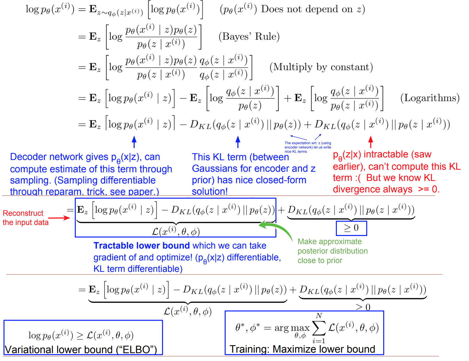
   In addition to decoder network modeling \(p_\theta(x\vert z)\), define additional encoder network \(q_\phi(z\vert x)\) that approximates \(p_\theta(z\vert x)\).
   This allows us to derive a lower bound on the data likelihood that is tractable, which we can optimize.
   

10. The Model:
    The Encoder (recognition/inference) and Decoder (generation) networks are probabilistic and output means and variances of each the conditionals respectively:
    

    The generation (forward-pass) is done via sampling as follows:
    

11. The Log-Likelihood of Data:
    Deriving the Log-Likelihood:
    

12. Training:
    Computing the bound (forward pass) for a given minibatch of input data:
    

13. Generation:
    

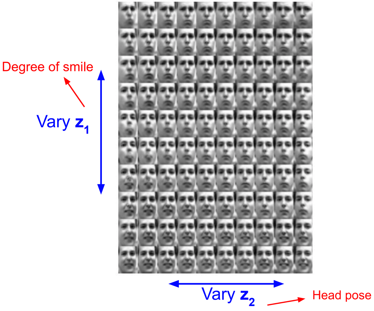
    - Diagonal prior on \(\boldsymbol{z} \implies\) independent latent variables
    - Different dimensions of \(\boldsymbol{z}\) encode interpretable factors of variation

    • Also good feature representation that can be computed using \(\mathrm{q}_ {\phi}(\mathrm{z} \vert \mathrm{x})\)!

    Examples:

    • MNIST:
      
    • CelebA:
      
14. Pros, Cons and Research:
    • Pros:
      • Principled approach to generative models
      • Allows inference of \(q(z\vert x)\), can be useful feature representation for other tasks
    • Cons:
      • Maximizing the lower bound of likelihood is okay, but not as good for evaluation as Auto-regressive models
      • Samples blurrier and lower quality compared to state-of-the-art (GANs)
    • Active areas of research:
      • More flexible approximations, e.g. richer approximate posterior instead of diagonal Gaussian
      • Incorporating structure in latent variables, e.g., Categorical Distributions