- Comprehensive list of activation functions in neural networks with pros/cons
- State Of The Art Activation Function: GELU, SELU, ELU, ReLU and more. With visualization of the activation functions and their derivatives (reddit!)
Introduction
-
Activation Functions:
In NNs, the activation function of a node defines the output of that node given an input or set of inputs.
The activation function is an abstraction representing the rate of action potential firing in the cell.
- Desirable Properties:
- Non-Linearity:
When the activation function is non-linear, then a two-layer neural network can be proven to be a universal function approximator. The identity activation function does not satisfy this property. When multiple layers use the identity activation function, the entire network is equivalent to a single-layer model. - Range:
When the range of the activation function is finite, gradient-based training methods tend to be more stable, because pattern presentations significantly affect only limited weights. When the range is infinite, training is generally more efficient because pattern presentations significantly affect most of the weights. In the latter case, smaller learning rates are typically necessary. - Continuously Differentiable:
This property is desirable for enabling gradient-based optimization methods. The binary step activation function is not differentiable at 0, and it differentiates to 0 for all other values, so gradient-based methods can make no progress with it. - Monotonicity:
- When the activation function is monotonic, the error surface associated with a single-layer model is guaranteed to be convex.
- During the training phase, backpropagation informs each neuron how much it should influence each neuron in the next layer. If the activation function isn’t monotonic then increasing the neuron’s weight might cause it to have less influence, the opposite of what was intended.
However, Monotonicity isn’t required. Several papers use non monotonic trained activation functions.
Gradient descent finds a local minimum even with non-monotonic activation functions. It might only take longer. - From a biological perspective, an “activation” depends on the sum of inputs, and once the sum surpasses a threshold, “firing” occurs. This firing should happen even if the sum surpasses the threshold by a small or a large amount; making monotonicity a desirable property to not limit the range of the “sum”.
- Smoothness with Monotonic Derivatives:
These have been shown to generalize better in some cases. - Approximating Identity near Origin:
Equivalent to \({\displaystyle f(0)=0}\) and \({\displaystyle f'(0)=1}\), and \({\displaystyle f'}\) is continuous at \(0\).
When activation functions have this property, the neural network will learn efficiently when its weights are initialized with small random values. When the activation function does not approximate identity near the origin, special care must be used when initializing the weights. - Zero-Centered Range:
Has effects of centering the data (zero mean) by centering the activations. Makes learning easier.
- Non-Linearity:
- Undesirable Properties:
- Saturation:
An activation functions output, with finite range, may saturate near its tail or head (e.g. \(\{0, 1\}\) for sigmoid). This leads to a problem called vanishing gradient. - Vanishing Gradients:
Happens when the gradient of an activation function is very small/zero. This usually happens when the activation function saturates at either of its tails.
The chain-rule will multiply the local gradient (of activation function) with the whole objective. Thus, when gradient is small/zero, it will “kill” the gradient \(\rightarrow\) no signal will flow through the neuron to its weights or to its data.
Slows/Stops learning completely. - Range Not Zero-Centered:
This is undesirable since neurons in later layers of processing in a Neural Network would be receiving data that is not zero-centered. This has implications on the dynamics during gradient descent, because if the data coming into a neuron is always positive (e.g. \(x>0\) elementwise in \(f=w^Tx+b\)), then the gradient on the weights \(w\) will during backpropagation become either all be positive, or all negative (depending on the gradient of the whole expression \(f\)). This could introduce undesirable zig-zagging dynamics in the gradient updates for the weights. However, notice that once these gradients are added up across a batch of data the final update for the weights can have variable signs, somewhat mitigating this issue. Therefore, this is an inconvenience but it has less severe consequences compared to the saturated activation problem above.
Makes optimization harder.
- Saturation:
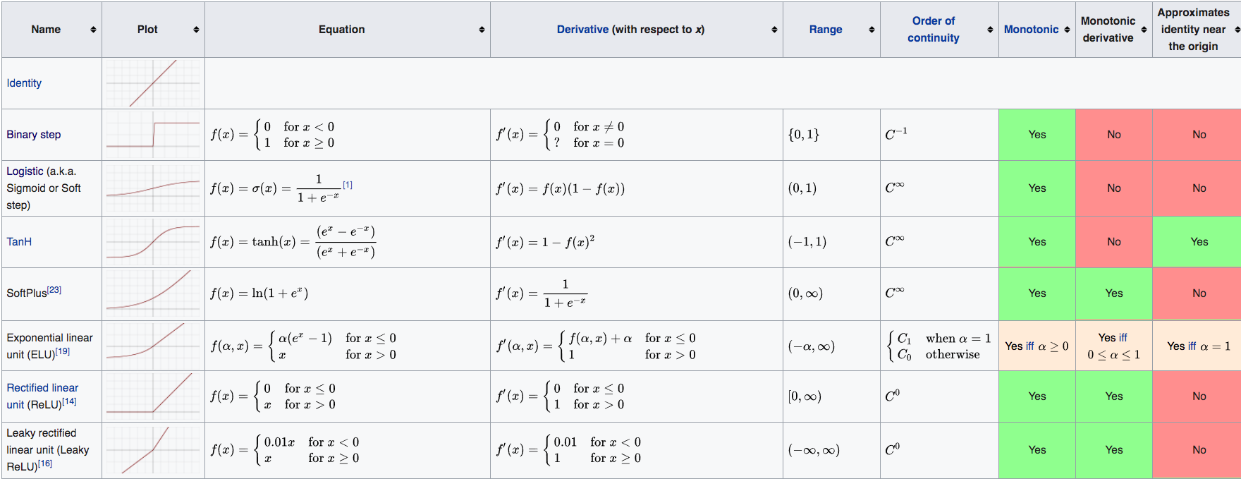
Activation Functions
- Sigmoid:
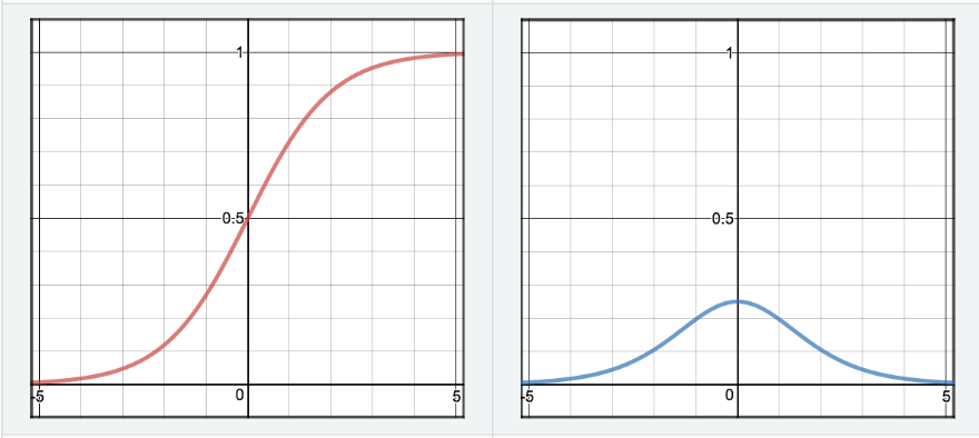
$$S(z)=\frac{1}{1+e^{-z}} \\ S^{\prime}(z)=S(z) \cdot(1-S(z))$$
Properties:
Never use as activation, use as an output unit for binary classification.- Pros:
- Has a nice interpretation as the firing rate of a neuron
- Cons:
- They Saturate and kill gradients \(\rightarrow\) Gives rise to vanishing gradients[^1] \(\rightarrow\) Stop Learning
- Happens when initialization weights are too large
- or sloppy with data preprocessing
- Neurons Activation saturates at either tail of \(0\) or \(1\)
- Output NOT Zero-Centered \(\rightarrow\) Gradient updates go too far in different directions \(\rightarrow\) makes optimization harder
- The local gradient \((z * (1-z))\) achieves maximum at \(0.25\), when \(z = 0.5\). \(\rightarrow\) very time the gradient signal flows through a sigmoid gate, its magnitude always diminishes by one quarter (or more) \(\rightarrow\) with basic SGD, the lower layers of a network train much slower than the higher one
- Pros:
- Tanh:
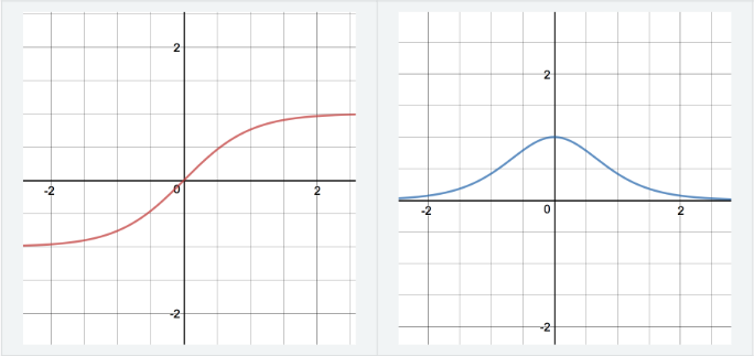
$$\tanh (z)=\frac{e^{z}-e^{-z}}{e^{z}+e^{-z}} \\ \tanh ^{\prime}(z)=1-\tanh (z)^{2}$$
Properties:
Strictly superior to Sigmoid (scaled version of sigmoid | stronger gradient). Good for activation.- Pros:
- Zero Mean/Centered
- Cons:
- They Saturate and kill gradients \(\rightarrow\) Gives rise to vanishing gradients[^1] \(\rightarrow\) Stop Learning
- They Saturate and kill gradients \(\rightarrow\) Gives rise to vanishing gradients[^1] \(\rightarrow\) Stop Learning
- Pros:
- ReLU:
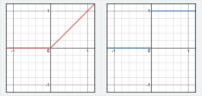
$$R(z)=\left\{\begin{array}{cc}{z} & {z>0} \\ {0} & {z<=0}\end{array}\right\} \\ R^{\prime}(z)=\left\{\begin{array}{ll}{1} & {z>0} \\ {0} & {z<0}\end{array}\right\}$$
Properties:
The best for activation (Better gradients).- Pros:
- Non-saturation of gradients which accelerates convergence of SGD
- Sparsity effects and induced regularization. discussion
ReLU (as usually used in neural networks) introduces sparsity in activations not in weights or biases. - Not computationally expensive
- Cons:
- ReLU not zero-centered problem:
The problem that ReLU is not zero-centered can be solved/mitigated by using batch normalization, which normalizes the signal before activation:From paper: We add the BN transform immediately before the nonlinearity, by normalizing \(x = Wu + b\); normalizing it is likely to produce activations with a stable distribution.
- Dying ReLUs (Dead Neurons):
If a neuron gets clamped to zero in the forward pass (it doesn’t “fire” / \(x<0\)), then its weights will get zero gradient. Thus, if a ReLU neuron is unfortunately initialized such that it never fires, or if a neuron’s weights ever get knocked off with a large update during training into this regime (usually as a symptom of aggressive learning rates), then this neuron will remain permanently dead. - cs231n Explanation
- Infinite Range:
Can blow up the activation.
- ReLU not zero-centered problem:
- Pros:
- Leaky-ReLU:
$$R(z)=\left\{\begin{array}{cc}{z} & {z>0} \\ {\alpha z} & {z<=0}\end{array}\right\} \\ R^{\prime}(z)=\left\{\begin{array}{ll}{1} & {z>0} \\ {\alpha} & {z<0}\end{array}\right\}$$
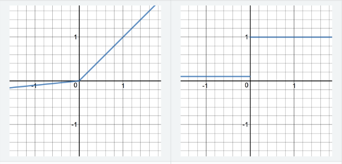
Properties:
Sometimes useful. Worth trying.- Pros:
- Leaky ReLUs are one attempt to fix the “dying ReLU” problem by having a small negative slope (of 0.01, or so).
- Cons:
The consistency of the benefit across tasks is presently unclear.
- Pros:
-
ELU:
<!–
-
Asynchronous:
-
Asynchronous:
–>
-
- Notes:
- It is very rare to mix and match different types of neurons in the same network, even though there is no fundamental problem with doing so.
- Identity Mappings:
When an activation function cannot achieve an identity mapping (e.g. ReLU map all negative inputs to zero); then adding extra depth actually decreases the best performance, in the case a shallower one would suffice (Deep Residual Net paper).
-
Softmax:
Motivation:
- Information Theory - from the perspective of information theory the softmax function can be seen as trying to minimize the cross-entropy between the predictions and the truth.
- Probability Theory - from this perspective since \(\hat{y}_ i\) represent log-probabilities we are in fact looking at the log-probabilities, thus when we perform exponentiation we end up with the raw probabilities. In this case the softmax equation find the MLE (Maximum Likelihood Estimate).
If a neuron’s output is a log probability, then the summation of many neurons’ outputs is a multiplication of their probabilities. That’s more commonly useful than a sum of probabilities. - It is a softened version of the argmax function (limit as \(T \rightarrow 0\))
Properties
- There is one nice attribute of Softmax as compared with standard normalisation:
It react to low stimulation (think blurry image) of your neural net with rather uniform distribution and to high stimulation (ie. large numbers, think crisp image) with probabilities close to 0 and 1.
While standard normalisation does not care as long as the proportion are the same.
Have a look what happens when soft max has 10 times larger input, ie your neural net got a crisp image and a lot of neurones got activated.
softmax([1,2]) # blurry image of a ferret
[0.26894142, 0.73105858]) # it is a cat perhaps !?
»> softmax([10,20]) # crisp image of a cat
[0.0000453978687, 0.999954602]) # it is definitely a CAT !And then compare it with standard normalisation:
std_norm([1,2]) # blurry image of a ferret
[0.3333333333333333, 0.6666666666666666] # it is a cat perhaps !?
»> std_norm([10,20]) # crisp image of a cat
[0.3333333333333333, 0.6666666666666666] # it is a cat perhaps !?
Notes: