Loss Functions (blog)
Information Theory (Cross-Entropy and MLE, MSE, Nash, etc.)
Loss Functions
Loss Functions
Abstractly, a loss function or cost function is a function that maps an event or values of one or more variables onto a real number, intuitively, representing some “cost” associated with the event.
Formally, a loss function is a function \(L :(\hat{y}, y) \in \mathbb{R} \times Y \longmapsto L(\hat{y}, y) \in \mathbb{R}\) that takes as inputs the predicted value \(\hat{y}\) corresponding to the real data value \(y\) and outputs how different they are.
Loss Functions for Regression
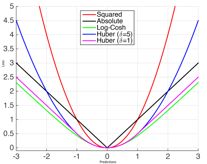
Introduction
Regression Losses usually only depend on the residual \(r = y - \hat{y}\) (i.e. what you have to add to your prediction to match the target)
Distance-Based Loss Functions:
A Loss function \(L(\hat{y}, y)\) is called distance-based if it:
- Only depends on the residual:
$$L(\hat{y}, y) = \psi(y-\hat{y}) \:\: \text{for some } \psi : \mathbb{R} \longmapsto \mathbb{R}$$
- Loss is \(0\) when residual is \(0\):
$$\psi(0) = 0$$
Translation Invariance:
Distance-based losses are translation-invariant:
$$L(\hat{y}+a, y+a) = L(\hat{y}, y)$$
Sometimes Relative-Error \(\dfrac{\hat{y}-y}{y}\) is a more natural loss but it is NOT translation-invariant
MSE
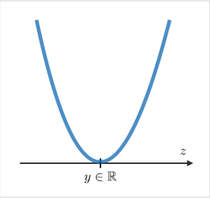
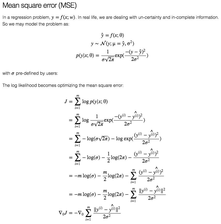
The MSE minimizes the sum of squared differences between the predicted values and the target values.
$$L(\hat{y}, y) = \dfrac{1}{n} \sum_{i=1}^{n}\left(y_{i}-\hat{y}_ {i}\right)^{2}$$
MAE
The MAE minimizes the sum of absolute differences between the predicted values and the target values.
$$L(\hat{y}, y) = \dfrac{1}{n} \sum_{i=1}^{n}\vert y_{i}-\hat{y}_ {i}\vert$$
Properties:
- Solution may be Non-unique
- Robustness to outliers
- Unstable Solutions:
The instability property of the method of least absolute deviations means that, for a small horizontal adjustment of a datum, the regression line may jump a large amount. The method has continuous solutions for some data configurations; however, by moving a datum a small amount, one could “jump past” a configuration which has multiple solutions that span a region. After passing this region of solutions, the least absolute deviations line has a slope that may differ greatly from that of the previous line. In contrast, the least squares solutions is stable in that, for any small adjustment of a data point, the regression line will always move only slightly; that is, the regression parameters are continuous functions of the data. - Data-points “Latching”1:
- Unique Solution:
If there are \(k\) features (including the constant), then at least one optimal regression surface will pass through \(k\) of the data points; unless there are multiple solutions. - Multiple Solutions:
The region of valid least absolute deviations solutions will be bounded by at least \(k\) lines, each of which passes through at least \(k\) data points.
- Unique Solution:
Huber Loss
AKA: Smooth Mean Absolute Error
$$L(\hat{y}, y) = \left\{\begin{array}{cc}{\frac{1}{2}(y-\hat{y})^{2}} & {\text { if }|(y-\hat{y})|<\delta} \\ {\delta(y-\hat{y})-\frac{1}{2} \delta} & {\text { otherwise }}\end{array}\right.$$
Properties:
- It’s less sensitive to outliers than the MSE as it treats error as square only inside an interval.
Code:
def Huber(yHat, y, delta=1.):
    return np.where(np.abs(y-yHat) < delta,.5*(y-yHat)**2 , delta*(np.abs(y-yHat)-0.5*delta))
KL-Divergence
$$L(\hat{y}, y) = $$
Analysis and Discussion
MSE vs MAE:
| MSE | MAE |
| Sensitive to outliers | Robust to outliers |
| Differentiable Everywhere | Non-Differentiable at \(0\) |
| Stable2 Solutions | Unstable Solutions |
| Unique Solution | Possibly multiple3 solutions |
- Statistical Efficiency:
- “For normal observations MSE is about \(12\%\) more efficient than MAE” - Fisher
- \(1\%\) Error is enough to make MAE more efficient
- 2/1000 bad observations, make the median more efficient than the mean
- Subgradient methods are slower than gradient descent
- you get a lot better convergence rate guarantees for MSE
Notes
Loss Functions for Classification
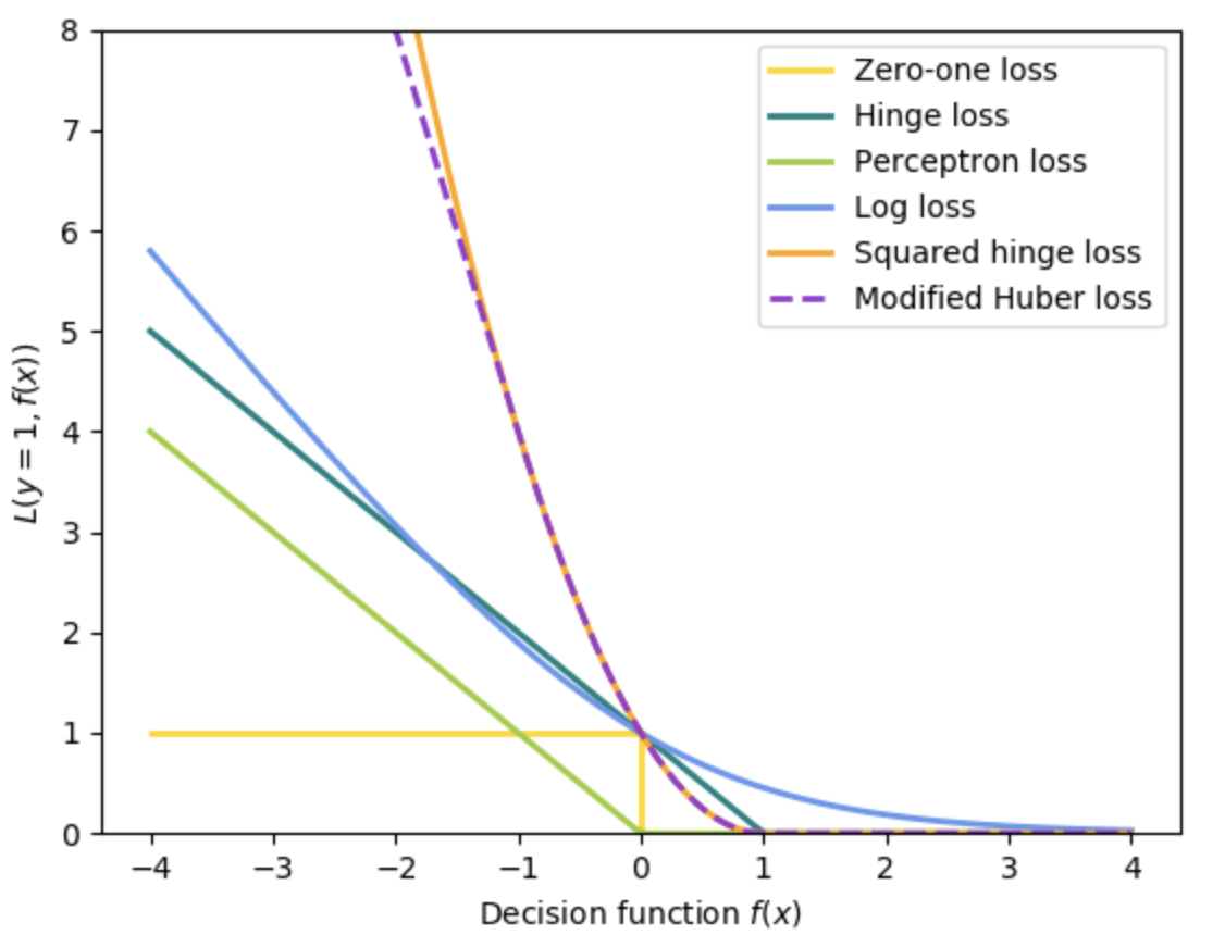
\(0-1\) Loss
$$L(\hat{y}, y) = I(\hat{y} \neq y) = \left\{\begin{array}{ll}{0} & {\hat{y}=y} \\ {1} & {\hat{y} \neq y}\end{array}\right.$$
MSE
We can write the loss in terms of the margin \(m = y\hat{y}\):
\(L(\hat{y}, y)=(y - \hat{y})^{2}=(1-y\hat{y})^{2}=(1-m)^{2}\)
Since \(y \in {-1,1} \implies y^2 = 1\)
$$L(\hat{y}, y) = (1-y \hat{y})^{2}$$


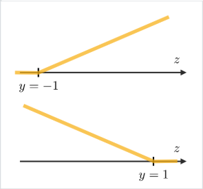
Hinge Loss
$$L(\hat{y}, y) = \max (0,1-y \hat{y})=|1-y \hat{y}|_ {+}$$
Properties:
- Continuous, Convex, Non-Differentiable
Logistic Loss
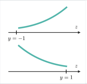
AKA: Log-Loss, Logarithmic Loss
$$L(\hat{y}, y) = \log{\left(1+e^{-y \hat{y}}\right)}$$
Properties:
- The logistic loss function does not assign zero penalty to any points. Instead, functions that correctly classify points with high confidence (i.e., with high values of \({\displaystyle \vert f({\vec {x}})\vert}\)) are penalized less. This structure leads the logistic loss function to be sensitive to outliers in the data.
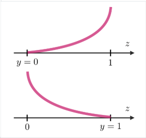
Cross-Entropy (Log Loss)
$$L(\hat{y}, y) = -\sum_{i} y_i \log \left(\hat{y}_ {i}\right)$$
Binary Cross-Entropy:
$$L(\hat{y}, y) = -\left[y \log \hat{y}+\left(1-y\right) \log \left(1-\hat{y}_ {n}\right)\right]$$
Cross-Entropy and Negative-Log-Probability:
The Cross-Entropy is equal to the Negative-Log-Probability (of predicting the true class) in the case that the true distribution that we are trying to match is peaked at a single point and is identically zero everywhere else; this is usually the case in ML when we are using a one-hot encoded vector with one class \(y = [0 \: 0 \: \ldots \: 0 \: 1 \: 0 \: \ldots \: 0]\) peaked at the \(j\)-th position
\(\implies\)
$$L(\hat{y}, y) = -\sum_{i} y_i \log \left(\hat{y}_ {i}\right) = - \log (\hat{y}_ {j})$$
Cross-Entropy and Log-Loss:
The Cross-Entropy is equal to the Log-Loss in the case of \(0, 1\) classification.
Equivalence of Binary Cross-Entropy and Logistic-Loss:
Given \(p \in\{y, 1-y\}\) and \(q \in\{\hat{y}, 1-\hat{y}\}\):
$$H(p,q)=-\sum_{x }p(x)\,\log q(x) = -y \log \hat{y}-(1-y) \log (1-\hat{y}) = L(\hat{y}, y)$$
- Notice the following property of the logistic function \(\sigma\) (used in derivation below):
\(\sigma(-x) = 1-\sigma(x)\)
Given:
- \(\hat{y} = \sigma(yf(x))\),4
- \(y \in \{-1, 1\}\),
- \(\hat{y}' = \sigma(f(x))\),
- \(y' = (1+y)/2 = \left\{\begin{array}{ll}{1} & {\text { for }} y' = 1 \\ {0} & {\text { for }} y = -1\end{array}\right. \in \{0, 1\}\)5
- We start with the modified binary cross-entropy
\(\begin{aligned} -y' \log \hat{y}'-(1-y') \log (1-\hat{y}') &= \left\{\begin{array}{ll}{-\log\hat{y}'} & {\text { for }} y' = 1 \\ {-\log(1-\hat{y}')} & {\text { for }} y' = 0\end{array}\right. \\ \\ &= \left\{\begin{array}{ll}{-\log\sigma(f(x))} & {\text { for }} y' = 1 \\ {-\log(1-\sigma(f(x)))} & {\text { for }} y' = 0\end{array}\right. \\ \\ &= \left\{\begin{array}{ll}{-\log\sigma(1\times f(x))} & {\text { for }} y' = 1 \\ {-\log(\sigma((-1)\times f(x)))} & {\text { for }} y' = 0\end{array}\right. \\ \\ &= \left\{\begin{array}{ll}{-\log\sigma(yf(x))} & {\text { for }} y' = 1 \\ {-\log(\sigma(yf(x)))} & {\text { for }} y' = 0\end{array}\right. \\ \\ &= \left\{\begin{array}{ll}{-\log\hat{y}} & {\text { for }} y' = 1 \\ {-\log\hat{y}} & {\text { for }} y' = 0\end{array}\right. \\ \\ &= -\log\hat{y} \\ \\ &= \log\left[\dfrac{1}{\hat{y}}\right] \\ \\ &= \log\left[\hat{y}^{-1}\right] \\ \\ &= \log\left[\sigma(yf(x))^{-1}\right] \\ \\ &= \log\left[ \left(\dfrac{1}{1+e^{-yf(x)}}\right)^{-1}\right] \\ \\ &= \log \left(1+e^{-yf(x)}\right)\end{aligned}\)
Cross-Entropy as Negative-Log-Likelihood (w/ equal probability outcomes):
Cross-Entropy and KL-Div:
When comparing a distribution \({\displaystyle q}\) against a fixed reference distribution \({\displaystyle p}\), cross entropy and KL divergence are identical up to an additive constant (since \({\displaystyle p}\) is fixed): both take on their minimal values when \({\displaystyle p=q}\), which is \({\displaystyle 0}\) for KL divergence, and \({\displaystyle \mathrm {H} (p)}\) for cross entropy.
Basically, minimizing either will result in the same solution.
Cross-Entropy VS MSE (& Classification Loss):
Basically, CE > MSE because the gradient of MSE \(z(1-z)\) leads to saturation when then output \(z\) of a neuron is near \(0\) or \(1\) making the gradient very small and, thus, slowing down training.
CE > Class-Loss because Class-Loss is binary and doesn’t take into account “how well” are we actually approximating the probabilities as opposed to just having the target class be slightly higher than the rest (e.g. \([c_1=0.3, c_2=0.3, c_3=0.4]\)).
Exponential Loss
$$L(\hat{y}, y) = e^{-\beta y \hat{y}}$$
Perceptron Loss
$${\displaystyle L(\hat{y}_i, y_i) = {\begin{cases}0&{\text{if }}\ y_i\cdot \hat{y}_i \geq 0\\-y_i \hat{y}_i&{\text{otherwise}}\end{cases}}}$$
Notes
- Logistic loss diverges faster than hinge loss (image). So, in general, it will be more sensitive to outliers. Reference. Bad info?
-
Reason is that the errors are equally weighted; so, tilting the regression line (within a region) will decrease the distance to a particular point and will increase the distance to other points by the same amount. ↩
-
\(f(x) = w^Tx\) in logistic regression ↩
-
We have to redefine the indicator/target variable to establish the equality. ↩