Object Detection

1. Object Detection:

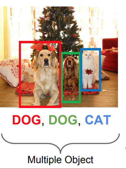
   Object Detection is the process of finding multiple instances of real-world objects such as faces, vehicles, and animals in images.

   

2. The Structure:

   • Input: Image
   • Output: A pair of (box-co-ords, class) of all the objects in a fixed number of classes that appear in the image.

3. Properties:

   In the problem of object detection, we normally do not know the number of objects that we need to detect.
   This leads to a problem when trying to model the problem as a regression problem due to the undefined number of coordinates of boxes.

   Thus, this problem is mainly modeled as a classification problem.

4. Applications:

   • Image Retrieval
   • Surveillance
   • Face Detection
   • Face Recognition
   • Pedestrian Detection
   • Self-Driving Cars

Approaches (The Pre-DeepLearning Era)

1. Semantic Texton Forests:

   This approach consists of ensembles of decision trees that act directly on image pixels.

   Semantic Texton Forests (STFs) are randomized decision forests that use only simple pixel comparisons on local image patches, performing both an implicit hierarchical clustering into semantic textons and an explicit local classification of the patch category.

   STFs allow us to build powerful texton codebooks without computing expensive filter-banks or descriptors, and without performing costly k-means clustering and nearest-neighbor assignment.

   Semantic Texton Forests for Image Categorization and Segmentation, Shawton et al. (2008)

2. Region Proposals:

   • Algorithm:
     • Find “blobby” image regions that are likely to contain objects

   These are relatively fast algorithms.

   Alexe et al, “Measuring the objectness of image windows”, TPAMI 2012
   Uijlings et al, “Selective Search for Object Recognition”, IJCV 2013
   Cheng et al, “BING: Binarized normed gradients for objectness estimation at 300fps”, CVPR 2014
   Zitnick and Dollar, “Edge boxes: Locating object proposals from edges”, ECCV 2014

3. Conditional Random Fields:

   CRFs provide a probabilistic framework for labeling and segmenting structured data.

   They try to model the relationship between pixels, e.g.:

   1. nearby pixels more likely to have same label
   2. pixels with similar color more likely to have same label
   3. the pixels above the pixels “chair” more likely to be “person” instead of “plane”
   4. refine results by iterations

   W. Wu, A. Y. C. Chen, L. Zhao and J. J. Corso (2014): “Brain Tumor detection and segmentation in a CRF framework with pixel-pairwise affinity and super pixel-level features”

   Plath et al. (2009): “Multi-class image segmentation using conditional random fields and global classification”

4. SuperPixel Segmentation:

   The concept of superpixels was first introduced by Xiaofeng Ren and Jitendra Malik in 2003.

   Superpixel is a group of connected pixels with similar colors or gray levels.
   They produce an image patch which is better aligned with intensity edges than a rectangular patch.

   Superpixel segmentation is the idea of dividing an image into hundreds of non-overlapping superpixels.
   Then, these can be fed into a segmentation algorithm, such as Conditional Random Fields or Graph Cuts, for the purpose of segmentation.

   Efficient graph-based image segmentation, Felzenszwalb, P.F. and Huttenlocher, D.P. International Journal of Computer Vision, 2004

   Quick shift and kernel methods for mode seeking, Vedaldi, A. and Soatto, S. European Conference on Computer Vision, 2008

   Peer Neubert & Peter Protzel (2014). Compact Watershed and Preemptive

Approaches (The Deep Learning Era)

1. The Sliding Window Approach:

   We utilize classification for detection purposes.

   • Algorithm:
     • We break up the input image into tiny “crops” of the input image.
     • Use Classification+Localization to find the class of the center pixel of the crop, or classify it as background.

       Using the same machinery for classification+Localization.

     • Slide the window and look at more “crops”

   Basically, we do classification+Localization on each crop of the image.

   • DrawBacks:
     • Very Inefficient and Expensive:
       We need to apply a CNN to a huge number of locations and scales.

   Sermant et. al 2013: “OverFeat”

2. Region Proposal Networks (R-CNNs):

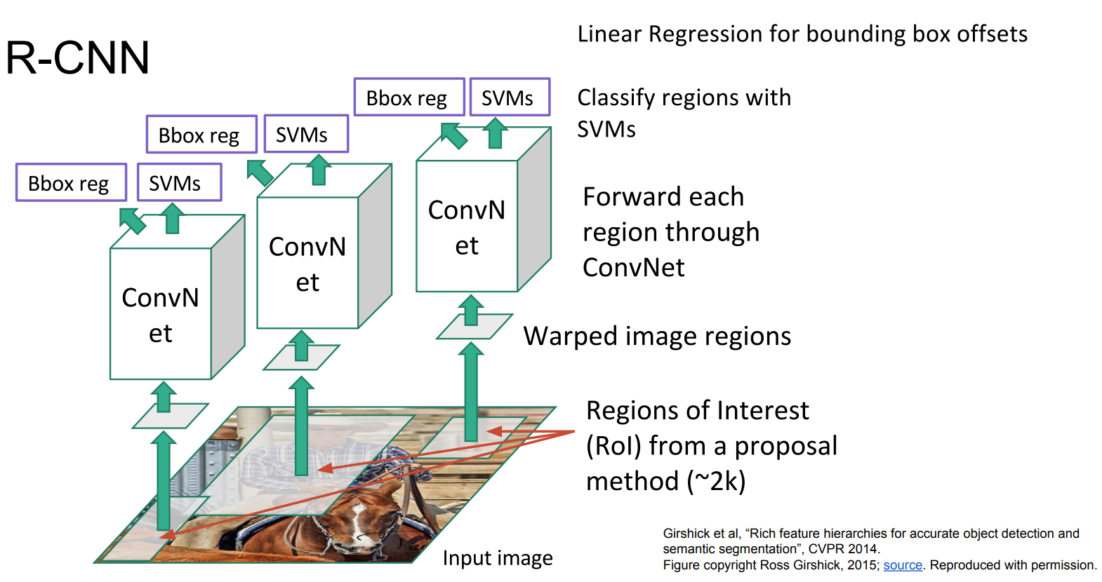
   A framework for object detection, that utilizes Region Proposals (Regions of Interest (ROIs)), consisting of three separate architectures.

   

   • Structure:
     • Input: Image vector
     • Output: A vector of bounding boxes coordinates and a class prediction for each box

   • Strategy:
     Propose a number of “bounding boxes”, then check if any of them, actually, corresponds to an object.

     The bounding boxes are created using Selective Search.

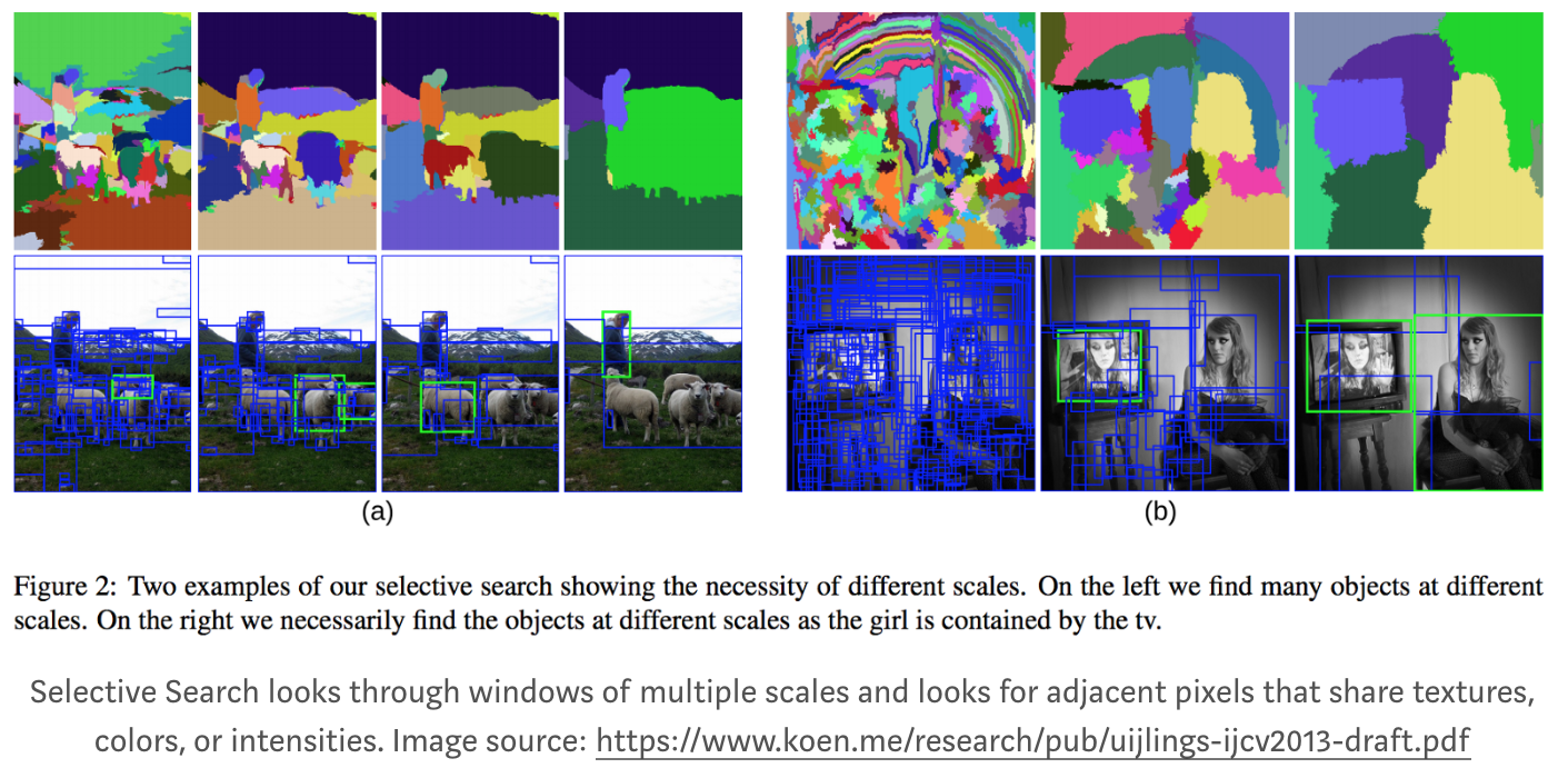
   • Selective Search: A method that looks at the image through windows of different sizes, and for each size tries to group together adjacent pixels by texture, color, or intensity to identify objects.
     

   • Key Insights:
     1. One can apply high-capacity convolutional neural networks (CNNs) to bottom-up region proposals in order to localize and segment objects
     2. When labeled training data is scarce, supervised pre-training for an auxiliary task, followed by domain-specific fine-tuning, yields a significant performance boost.

   • Algorithm:
     • Create Region Proposals (Regions of Interest (ROIs)) of bounding boxes
     • Warp the regions to a standard square size to fit the “cnn classification models”, due to the FCNs
     • Pass the warped images to a modified version of AlexNet to extract image features
     • Pass the image features to an SVM to classify the image regions into a class or background
     • Run the bounding box coordinates in a Linear Regression model to “tighten” the bounding boxes
       • Linear Regression:
         • Structure:
           • Input: sub-regions of the image corresponding to objects
           • Output: New bounding box coordinates for the object in the sub-region.

   • Issues:
     • Ad hoc training objectives:
       • Fine-tune network with softmax classifier (log loss)
       • Train post-hoc linear SVMs (hinge loss)
       • Train post-hoc bounding-box regressions (least squares)
     • Training is slow (84h), takes a lot of disk space
     • Inference (detection) is slow
       • 47s / image with VGG16 [Simonyan & Zisserman. ICLR15]
       • Fixed by SPP-net [He et al. ECCV14]

   R-CNN is slow because it performs a ConvNet forward pass for each region proposal, without sharing computation.

   R. Girshick, J. Donahue, T. Darrell, J. Malik. (2014): “Rich feature hierarchies for accurate object detection and semantic segmentation”

3. Fast R-CNNs:

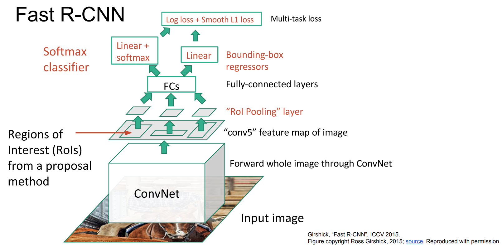
   A single, end-to-end, architecture for object detection based on R-CNNs, that vastly improves on its speed and accuracy by utilizing shared computations of features.

   

   • Structure:
     • Input: Image vector
     • Output: A vector of bounding boxes coordinates and a class prediction for each box

   • Key Insights:
     1. Instead of running the ConvNet on each region proposal separately, we run the ConvNet on the entire image.
     2. Instead of taking crops of the original image, we project the regions of interest onto the ConvNet Feature Map, corresponding to each RoI, and then use the projected regions in the feature map for classification.
        This allows us to reuse a lot of the expensive computation of the features.
     3. Jointly train the CNN, classifier, and bounding box regressor in a single model. Where earlier we had different models to extract image features (CNN), classify (SVM), and tighten bounding boxes (regressor), Fast R-CNN instead used a single network to compute all three.

   • Algorithm:
     • Create Region Proposals (Regions of Interest (ROIs)) of bounding boxes
     • Pass the entire image to a modified version of AlexNet to extract image features by creating an image feature map for the entire image.
     • Project each RoI to the feature map and crop each respective projected region
     • Apply RoI Pooling to the regions extracted from the feature map to a standard square size to fit the “cnn classification models”, due to the FCNs
     • Pass the image features to an SVM to classify the image regions into a class or background
     • Run the bounding box coordinates in a Linear Regression model to “tighten” the bounding boxes
       • Linear Regression:
         • Structure:
           • Input: sub-regions of the image corresponding to objects
           • Output: New bounding box coordinates for the object in the sub-region.

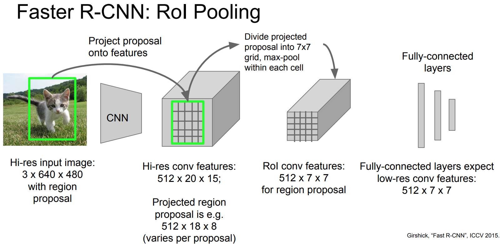
   • RoI Pooling: is a pooling technique aimed to perform max pooling on inputs of nonuniform sizes to obtain fixed-size feature maps (e.g. 7×7).
     • Structure:
       • Input: A fixed-size feature map obtained from a deep convolutional network with several convolutions and max pooling layers.
       • Output: An N x 5 matrix of representing a list of regions of interest, where N is a number of RoIs. The first column represents the image index and the remaining four are the coordinates of the top left and bottom right corners of the region.
         For every region of interest from the input list, it takes a section of the input feature map that corresponds to it and scales it to some pre-defined size.
     • Scaling:
       1. Divide the RoI into equal-sized sections (the number of which is the same as the dimension of the output)
       2. Find the largest value in each section
       3. Copy these max values to the output buffer
          The dimension of the output is determined solely by the number of sections we divide the proposal into.
          

   • The Bottleneck:
     It appears that Fast R-CNNs are capable of object detection at test time in:
     • Including RoIs: 2.3s
     • Excluding RoIs: 0.3s
       Thus, the bottleneck for the speed seems to be the method of creating the RoIs, Selective Search

   [1] Girshick, Ross (2015). “Fast R-CNN”

4. Faster R-CNNs:

   A single, end-to-end, architecture for object detection based on Fast R-CNNs, that tackles the bottleneck in speed (i.e. computing RoIs) by introducing Region Proposal Networks (RPNs) to make a CNN predict proposals from features.
   Region Proposal Networks share full-image convolutional features with the detection network, thus enabling nearly cost-free region proposals.
   The network is jointly trained with 4 losses: 1. RPN classify object / not object 2. RPN regress box coordinates 3. Final classification score (object classes) 4. Final box coordinates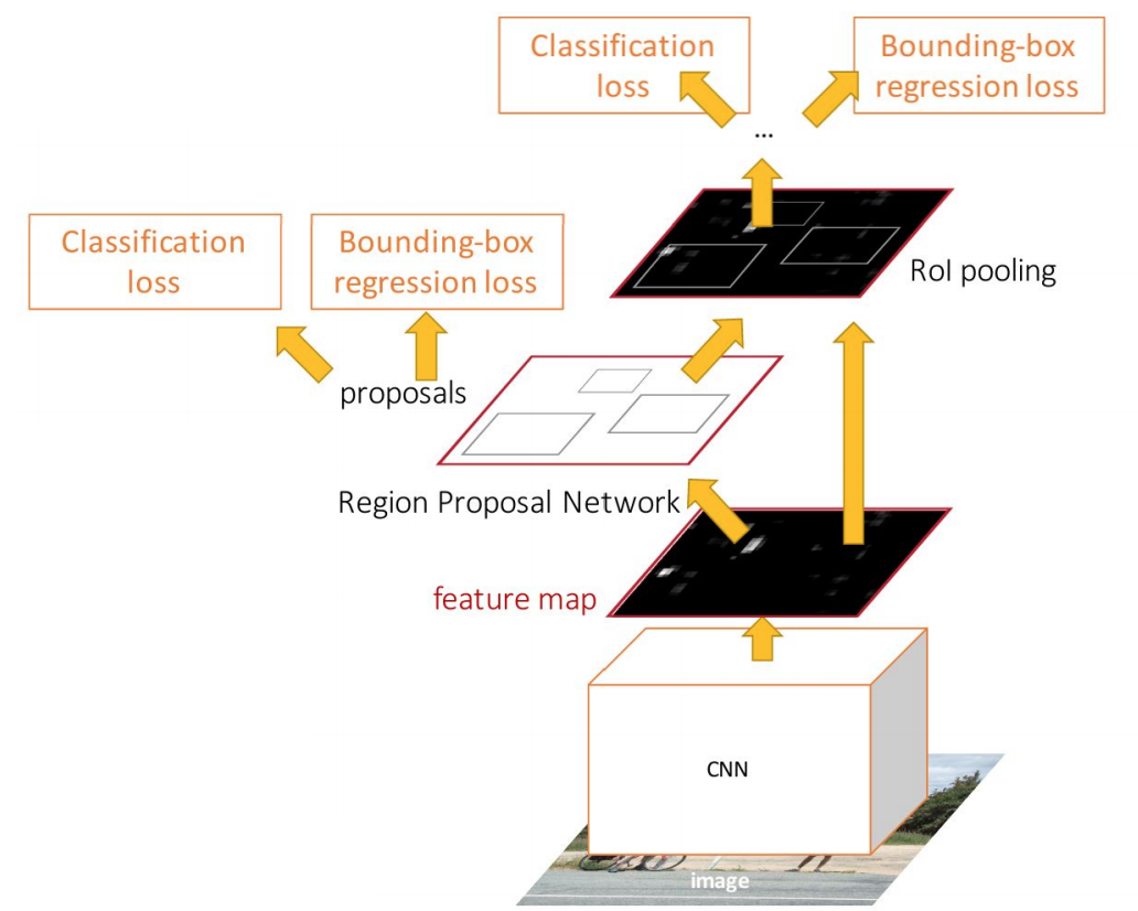

   

   • Region Proposal Network (RPN): is an, end-to-end, fully convolutional network that simultaneously predicts object bounds and objectness scores at each position.
     RPNs work by passing a sliding window over the CNN feature map and at each window, outputting k potential bounding boxes and scores for how good each of those boxes is expected to be.

   • Structure:
     • Input: Image vector
     • Output: A vector of bounding boxes coordinates and a class prediction for each box

   • Key Insights:
     1. Replace Selective Search for finding RoIs by a Region Proposal Network that shares the features, and thus reduces the computation and time, of the pipeline.

   • Algorithm:
     • Pass the entire image to a modified version of AlexNet to extract image features by creating an image feature map for the entire image.
     • Pass the CNN Feature Map to the RPN to generate bounding boxes and a score for each bounding box
     • Pass each such bounding box that is likely to be an object into Fast R-CNN to generate a classification and tightened bounding boxes.

   Ren et al, (2015). “Faster R-CNN: Towards Real-Time Object Detection with Region Proposal Networks”

Methods, Approaches and Algorithms in Training DL Models