Learning Deep Generative Models (pdf)
AutoRegressive Models (CS236 pdf)
Deep Generative Models (CS236 pdf)
Deep Generative Models (Lecture)
CS294 Berkeley - Deep Unsupervised Learning

Unsupervised Learning

1. Unsupervised Learning:
   Data: \(x\) Just data, no labels!
   Goal: Learn some underlying hidden structure of the data
   Examples: Clustering, dimensionality reduction, feature learning, density estimation, etc.
   
   

Generative Models

Given some data \(\{(d,c)\}\) of paired observations \(d\) and hidden classes \(c\):

1. Generative (Joint) Models:
   Generative Models are Joint Models.
   Joint Models place probabilities \(\left(P(c,d)\right)\) over both the observed data and the “target” (hidden) variables that can only be computed from those observed.

   Generative models are typically probabilistic, specifying a joint probability distribution (\(P(d,c)\)) over observation and target (label) values, and tries to Maximize this joint Likelihood.

   Choosing weights turn out to be trivial: chosen as the relative frequencies.

   They address the problem of density estimation, a core problem in unsupervised learning.

   Examples:

   • Gaussian Mixture Model
   • Naive Bayes Classifiers
   • Hidden Markov Models (HMMs)
   • Restricted Boltzmann Machines (RBMs)
   • AutoEncoders
   • Generative Adversarial Networks (GANs)

2. Discriminative (Conditional) Models:

   Discriminative Models are Conditional Models.

   Conditional Models provide a model only for the “target” (hidden) variabless.
   They take the data as given, and put a probability \(\left(P(c \vert d)\right)\) over the “target” (hidden) structures given the data.

   Conditional Models seek to Maximize the Conditional Likelihood.

   This (maximization) task is usually harder to do.

   Examples:

   • Logistic Regression
   • Conditional LogLinear/Maximum Entropy Models
   • Condtional Random Fields
   • SVMs
   • Perceptrons
   • Neural Networks

3. Generative VS Discriminative Models:
   Basically, Discriminative Models infer outputs based on inputs,
   while Generative Models generate, both, inputs and outputs (typically given some hidden paramters).

   However, notice that the two models are usually viewed as complementary procedures.
   One does not necessarily outperform the other, in either classificaiton or regression tasks.

4. Example Uses of Generative Models:

   • Clustering
   • Dimensionality Reduction
   • Feature Learning
   • Density Estimation

5. Density Estimation:

   Generative Models, given training data, will generate new samples from the same distribution.

   They address the Density Estimation problem, a core problem in unsupervised learning.

   • Types of Density Estimation:
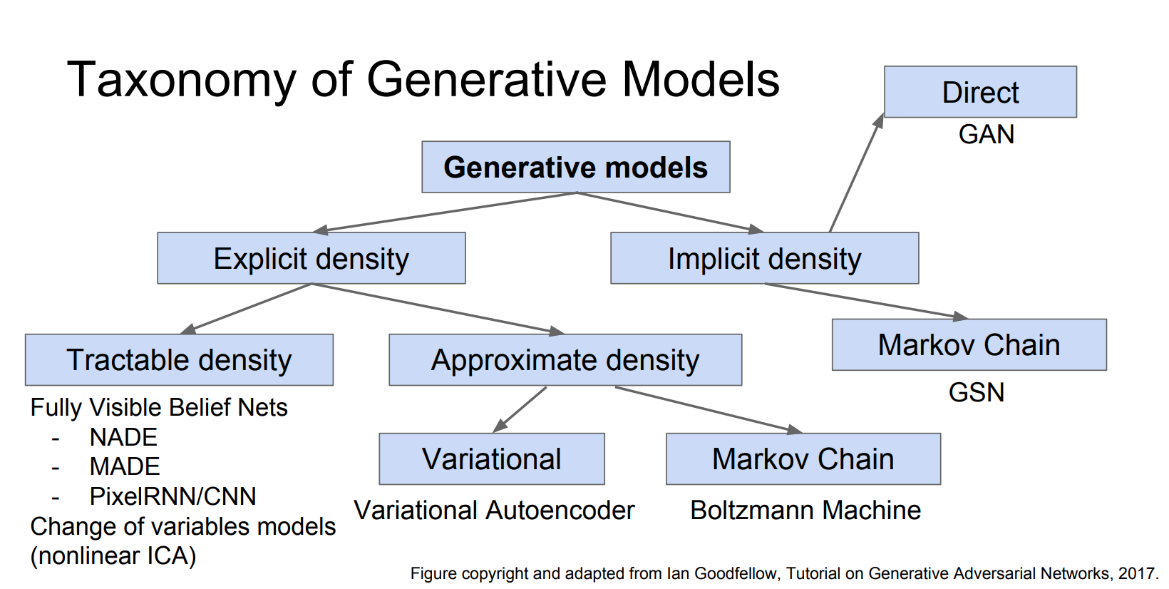
     • Explicit: Explicitly define and solve for \(p_\text{model}(x)\)
     • Implicit: Learn model that can sample from \(p_\text{model}(x)\) without explicitly defining it

6. Applications of Generative Models:

   • Realistic samples for artwork
   • Super-Resolution
   • Colorization
   • Generative models of time-series data can be used for simulation and planning

     reinforcement learning applications

   • Inference of Latent Representations that can be useful as general feature descriptors

7. Taxonomy of Generative Models:

   

AutoRegressive Models - PixelRNN and PixelCNN

AutoRegressive Models (pdf)

1. Fully Visible (Deep) Belief Networks:
   Deep Belief Network (DBNs) are generative graphical models, or alternatively a class of deep neural networks, composed of multiple layers of latent variables (“hidden units”), with connections between the layers but not between units within each layer.

   DBNs undergo unsupervised training to learn to probabilistically reconstruct the inputs.

   They generate an Explicit Density Model.

   They use the chain rule to decompose the _likelihood of an image \(x\) into products of 1-d distributions:
   
   then, they Maximize the Likelihood of the training data.

   The conditional distributions over pixels are very complex.
   We model them using a neural network.

2. PixelRNN:

   is a proposed architecture (part of the class of Auto-Regressive models) to model an explicit distribution of natural images in an expressive, tractable, and scalable way.

   It sequentially predicts the pixels in an image along two spatial dimensions.

   The Method models the discrete probability of the raw pixel values and encodes the complete set of dependencies in an image.

   The approach is to use probabilistic density models (like Gaussian or Normal distribution) to quantify the pixels of an image as a product of conditional distributions.
   This approach turns the modeling problem into a sequence problem where the next pixel value is determined by all the previously generated pixel values.

   • Key Insights:
     • Generate image pixels starting from corner
     • Dependency on previous pixels is modeled using an LSTM

   

   • The Model:
     • Scan the image, one row at a time and one pixel at a time (within each row)
     • Given the scanned content, predict the distribution over the possible values for the next pixel
     • Joint distribution over the pixel values is factorized into a product of conditional distributions thus causing the problem as a sequence problem
     • Parameters used in prediction are shared across all the pixel positions
     • Since each pixel is jointly determined by 3 values (3 colour channels), each channel may be conditioned on other channels as well

   • Drawbacks:
     • Sequential training is slow
     • Sequential generation is slow

   Further Reading

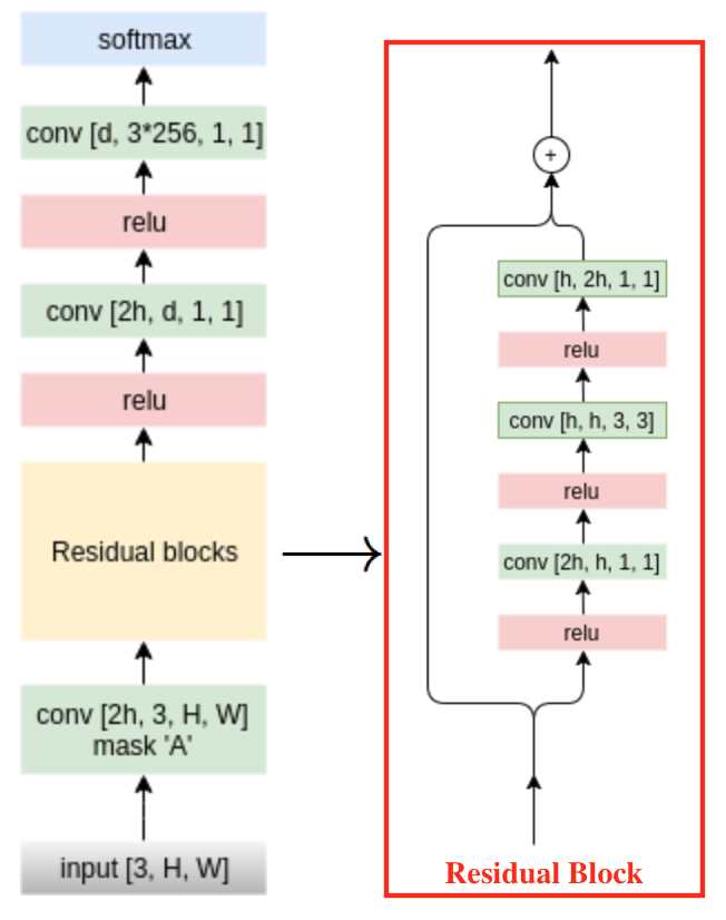
3. PixelCNN:

   Similar to the PixelRNN model, the PixelCNN models the Pixel Distribution \(p(\vec{x})\), where \(\vec{x} = (x_0, \ldots, x_n)\) is the vector of pixel values of a given image.

   Similarly, we use the chain rule for join distribution: \(p(x) = p(x_0) \prod_1^n p(x_i | x_{i<})\).

   such that, the first pixel is independent, the second depends on the first, and the third depends on, both, the first and second, etc.

   

   • Key Insights:
     • Still generate image pixels starting from corner
     • Dependency on previous pixels now modeled using a CNN over context region
     • Training: maximize likelihood of training images

   • Upsides:
     • Training is faster than PixelRNN: since we can parallelize the convolutions because the context region values are known from the training images.

   • Issues:
     • Generation is still sequential, thus, slow.

   Further Reading

4. Improving PixelCNN Performance:
   • Gated Convolutional Layers
   • Short-cut connections
   • Discretized logistic loss
   • Multi-scale
   • Training tricks

   Further Reading:

   • PixelCNN++ | Salimans et al. 2017
   • Van der Oord et al. NIPS 2016
   • Pixel-Snail
5. Pros and Cons of Auto-Regressive Models:
   • Pros:
     • Can explicitly compute likelihood \(p(x)\)
     • Explicit likelihood of training data gives good evaluation metric
     • Good Samples
   • Cons:
     • Sequential Generation is Slow

Variational Auto-Encoders

Auto-Encoders (click to read more) are unsupervised learning methods that aim to learn a representation (encoding) for a set of data in a smaller dimension.
Auto-Encoders generate Features that capture factors of variation in the training data.

1. Auto-Regressive Models VS Variational Auto-Encoders:

   Auto-Regressive Models defined a tractable (discrete) density function and, then, optimized the likelihood of training data:

   \[p_\theta(x) = p(x_0) \prod_1^n p(x_i | x_{i<})\]

   On the other hand, VAEs defines an intractable (continuous) density function with latent variable \(z\):

   \[p_\theta(x) = \int p_\theta(z) p_\theta(x|z) dz\]

   but cannot optimize directly; instead, derive and optimiz a lower bound on likelihood instead.

2. Variational Auto-Encoders (VAEs):

   Variational Autoencoder models inherit the autoencoder architecture, but make strong assumptions concerning the distribution of latent variables.

   They use variational approach for latent representation learning, which results in an additional loss component and specific training algorithm called Stochastic Gradient Variational Bayes (SGVB).

3. Assumptions:

   VAEs assume that:

   • The data is generated by a directed graphical model \(p(x\vert z)\)
   • The encoder is learning an approximation \(q_\phi(z|x)\) to the posterior distribution \(p_\theta(z|x)\)
     where \({\displaystyle \mathbf {\phi } }\) and \({\displaystyle \mathbf {\theta } }\) denote the parameters of the encoder (recognition model) and decoder (generative model) respectively.
   • The training data \(\left\{x^{(i)}\right\}_{i=1}^N\) is generated from underlying unobserved (latent) representation \(\mathbf{z}\)

4. The Objective Function:

   \[{\displaystyle {\mathcal {L}}(\mathbf {\phi } ,\mathbf {\theta } ,\mathbf {x} )=D_{KL}(q_{\phi }(\mathbf {z} |\mathbf {x} )||p_{\theta }(\mathbf {z} ))-\mathbb {E} _{q_{\phi }(\mathbf {z} |\mathbf {x} )}{\big (}\log p_{\theta }(\mathbf {x} |\mathbf {z} ){\big )}}\]

   where \({\displaystyle D_{KL}}\) is the Kullback–Leibler divergence (KL-Div).

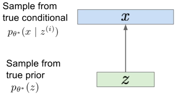
5. The Generation Process:

   

6. The Goal:

   The goal is to estimate the true parameters \(\theta^\ast\) of this generative model.

7. Representing the Model:

   • To represent the prior \(p(z)\), we choose it to be simple, usually Gaussian
   • To represent the conditional (which is very complex), we use a neural-network

8. Intractability:

   The Data Likelihood:

   \[p_\theta(x) = \int p_\theta(z) p_\theta(x|z) dz\]

   is intractable to compute for every \(z\).

   Thus, the Posterior Density:

   \[p_\theta(z|x) = \dfrac{p_\theta(x|z) p_\theta(z)}{p_\theta(x)} = \dfrac{p_\theta(x|z) p_\theta(z)}{\int p_\theta(z) p_\theta(x|z) dz}\]

   is, also, intractable

9. Dealing with Intractability:

   In addition to decoder network modeling \(p_\theta(x\vert z)\), define additional encoder network \(q_\phi(z\vert x)\) that approximates \(p_\theta(z\vert x)\)

   This allows us to derive a lower bound on the data likelihood that is tractable, which we can optimize.

10. The Model:

    • The Encoder (recognition/inference) and Decoder (generation) networks are probabilistic and output means and variances of each the conditionals respectively:
      
    • The generation (forward-pass) is done via sampling as follows:
      

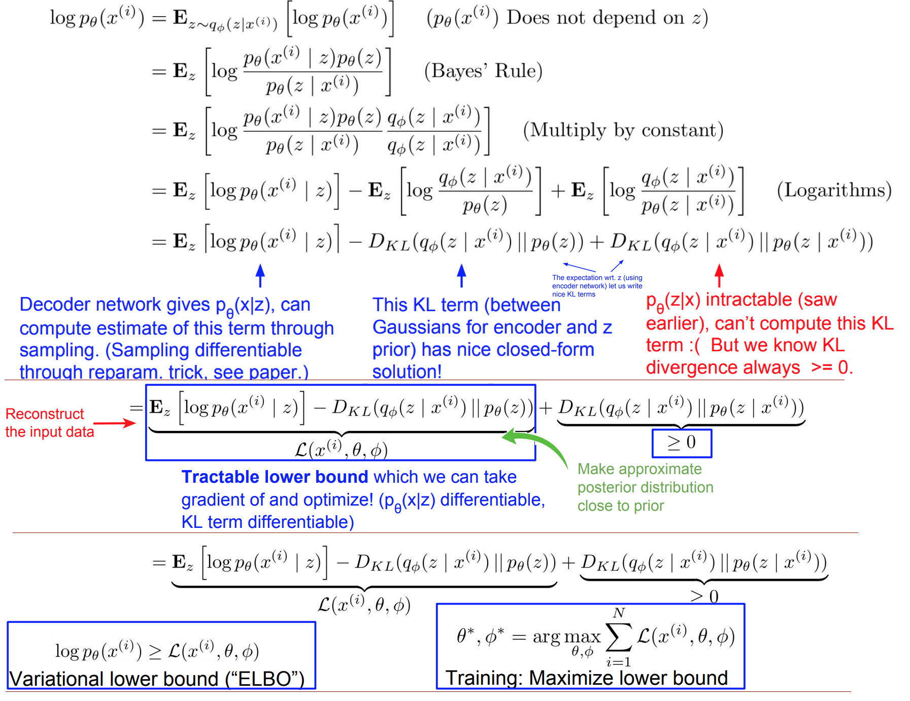
11. The Log-Likelihood of Data:

    • Deriving the Log-Likelihood:

    

12. Training the Model:

13. Pros, Cons and Research:

    • Pros:
      • Principled approach to generative models
      • Allows inference of \(q(z\vert x)\), can be useful feature representation for other tasks

    • Cons:
      • Maximizing the lower bound of likelihood is okay, but not as good for evaluation as Auto-regressive models
      • Samples blurrier and lower quality compared to state-of-the-art (GANs)

    • Active areas of research:
      • More flexible approximations, e.g. richer approximate posterior instead of diagonal Gaussian
      • Incorporating structure in latent variables

Generative Adversarial Networks (GANs)

1. Auto-Regressive Models VS Variational Auto-Encoders VS GANs:

   Auto-Regressive Models defined a tractable (discrete) density function and, then, optimized the likelihood of training data:

   \[p_\theta(x) = p(x_0) \prod_1^n p(x_i | x_{i<})\]

   While VAEs defined an intractable (continuous) density function with latent variable \(z\):

   \[p_\theta(x) = \int p_\theta(z) p_\theta(x|z) dz\]

   but cannot optimize directly; instead, derive and optimize a lower bound on likelihood instead.

   On the other hand, GANs rejects explicitly defining a probability density function, in favor of only being able to sample.

2. Generative Adversarial Networks:

   are a class of AI algorithms used in unsupervised machine learning, implemented by a system of two neural networks contesting with each other in a zero-sum game framework.

3. Motivation:

   • Problem: we want to sample from complex, high-dimensional training distribution; there is no direct way of doing this.
   • Solution: we sample from a simple distribution (e.g. random noise) and learn a transformation that maps to the training distribution, by using a neural network.

   • Generative VS Discriminative: discriminative models had much more success because deep generative models suffered due to the difficulty of approximating many intractable probabilistic computations that arise in maximum likelihood estimation and related strategies, and due to difficulty of leveraging the benefits of piecewise linear units in the generative context.
     GANs propose a new framework for generative model estimation that sidesteps these difficulties.

4. Structure:

   • Goal: estimating generative models that capture the training data distribution
   • Framework: an adversarial process in which two models are simultaneously trained a generative model \(G\) that captures the data distribution, and a discriminative model \(D\) that estimates the probability that a sample came from the training data rather than \(G\).
   • Training:
     • \(G\) maximizes the probability of \(D\) making a mistake