• Building an LSTM from Scratch in PyTorch
• Exploring LSTMs, their Internals and How they Work (Blog!)

GRUs

1. Gated Recurrent Units:
   Gated Recurrent Units (GRUs) are a class of modified (Gated) RNNs that allow them to combat the vanishing gradient problem by allowing them to capture more information/long range connections about the past (memory) and decide how strong each signal is.
   
   

2. Main Idea:
   Unlike standard RNNs which compute the hidden layer at the next time step directly first, GRUs computes two additional layers (gates) (Each with different weights):

   • Update Gate:

     $$z_t = \sigma(W^{(z)}x_t + U^{(z)}h_{t-1})$$

   • Reset Gate:

     $$r_t = \sigma(W^{(r)}x_t + U^{(r)}h_{t-1})$$

   The Update Gate and Reset Gate computed, allow us to more directly influence/manipulate what information do we care about (and want to store/keep) and what content we can ignore.

   We can view the actions of these gates from their respecting equations as:

   • New Memory Content:
     at each hidden layer at a given time step, we compute some new memory content,
     if the reset gate \(= \approx 0\), then this ignores previous memory, and only stores the new word information.

     $$ \tilde{h}_ t = \tanh(Wx_t + r_t \odot Uh_{t-1})$$

   • Final Memory:
     the actual memory at a time step \(t\), combines the Current and Previous time steps,
     if the update gate \(= \approx 0\), then this, again, ignores the newly computed memory content, and keeps the old memory it possessed.

     $$h_ t = z_ t \odot h_ {t-1} + (1-z_t) \odot \tilde{h}_ t$$

Long Short-Term Memory

1. LSTM:
   The Long Short-Term Memory (LSTM) Network is a special case of the Recurrent Neural Network (RNN) that uses special gated units (a.k.a LSTM units) as building blocks for the layers of the RNN.

   LSTM Equations:

   $$\begin{align} f_{t}&=\sigma_{g}\left(W_{f} x_{t}+U_{f} h_{t-1}+b_{f}\right) \\ i_{t}&=\sigma_{g}\left(W_{i} x_{t}+U_{i} h_{t-1}+b_{i}\right) \\ o_{t}&=\sigma_{g}\left(W_{o} x_{t}+U_{o} h_{t-1}+b_{o}\right) \\ c_{t}&=f_{t} \circ c_{t-1}+i_{t} \circ \sigma_{c}\left(W_{c} x_{t}+U_{c} h_{t-1}+b_{c}\right) \\ h_{t}&=o_{t} \circ \sigma_{h}\left(c_{t}\right) \end{align}$$

   where:
   \(\sigma_{g}\): sigmoid function.
   \({\displaystyle \sigma_{c}}\): hyperbolic tangent function.
   \({\displaystyle \sigma_{h}}\): hyperbolic tangent function or, as the peephole LSTM paper suggests, \({\displaystyle \sigma_{h}(x)=x}\).
   
   

2. Architecture:
   The LSTM, usually, has four gates:
   • Input Gate:
     The input gate determines how much does the current input vector (current cell) matters
     It controls the extent to which a new value flows into the cell

     $$i_t = \sigma(W^{(i)}x_t + U^{(i)}h_{t-1})$$

   • Forget Gate:
     Determines how much of the past memory, that we have kept, is still needed
     It controls the extent to which a value remains in the cell

     $$f_t = \sigma(W^{(f)}x_t + U^{(f)}h_{t-1})$$

   • Output Gate: Determines how much of the current cell matters for our current prediction (i.e. passed to the sigmoid)
     It controls the extent to which the value in the cell is used to compute the output activation of the LSTM unit

     $$o_t = \sigma(W^{(o)}x_t + U^{(o)}h_{t-1})$$

   • Memory Cell: The memory cell is the cell that contains the short-term memory collected from each input

     $$\begin{align} \tilde{c}_t & = \tanh(W^{(c)}x_t + U^{(c)}h_{t-1}) & \text{New Memory} \\ c_t & = f_t \odot c_{t-1} + i_t \odot \tilde{c}_ t & \text{Final Memory} \end{align}$$

     The Final Hidden State is calculated as follows:

     $$h_t = o_t \odot \sigma(c_t)$$

3. Properties:
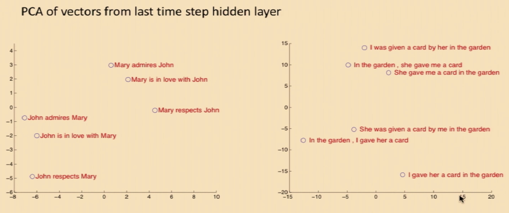
   • Syntactic Invariance:
     When one projects down the vectors from the last time step hidden layer (with PCA), one can observe the spatial localization of syntacticly-similar sentences
     

LSTMS:

• The core of the history/memory is captured in the cell-state \(c_{n}\) instead of the hidden state \(h_{n}\).
• (&) Key Idea: The update to the cell-state \(c_{n}=c_{n-1}+\operatorname{tanh}\left(V\left[w_{n-1} ; h_{n-1}\right]+b_{c}\right)\) here are additive. (differentiating a sum gives the identity) Making the gradient flow nicely through the sum. As opposed to the multiplicative updates to \(h_n\) in vanilla RNNs.

  There is non-linear funcs applied to the history/context cell-state. It is composed of linear functions. Thus, avoids gradient shrinking.

• In the recurrency of the LSTM the activation function is the identity function with a derivative of 1.0. So, the backpropagated gradient neither vanishes or explodes when passing through, but remains constant.
• By the selective read, write and forget mechanism (using the gating architecture) of LSTM, there exist at least one path, through which gradient can flow effectively from \(L\) to \(\theta\). Hence no vanishing gradient.
• However, one must remember that, this is not the case for exploding gradient. It can be proved that, there can exist at-least one path, thorough which gradient can explode.
• LSTM decouples cell state (typically denoted by c) and hidden layer/output (typically denoted by h), and only do additive updates to c, which makes memories in c more stable. Thus the gradient flows through c is kept and hard to vanish (therefore the overall gradient is hard to vanish). However, other paths may cause gradient explosion.
• The Vanishing gradient solution for LSTM is known as Constant Error Carousel.
• Why can RNNs with LSTM units also suffer from “exploding gradients”?

• Lecture on gradient flow paths through gates

• LSTMs (Lec Oxford)

Important Links:
The unreasonable effectiveness of Character-level Language Models
character-level language model with a Vanilla Recurrent Neural Network, in Python/numpy
Visualizing and Understanding Recurrent Networks - Karpathy Lec
Cool LSTM Diagrams - blog
Illustrated Guide to Recurrent Neural Networks: Understanding the Intuition
Code LSTM in Python
Mikolov Thesis: STATISTICAL LANGUAGE MODELS BASED ON NEURAL NETWORKS