Ahmad Badary

Sequence to Sequence Learning with Neural Network

Towards End-to-End Speech Recognition with Recurrent Neural Networks

Attention-Based Models for Speech Recognition

Attention Is All You Need

Sequence to Sequence Learning with Neural Network

Introduction:
This paper presents a general end-to-end approach to sequence learning that makes minimal assumptions (Domain-Independent) on the sequence structure.
It introduces Seq2Seq.
Structure:
- Input: sequence of input vectors
- Output: sequence of output labels
Strategy:
The idea is to use one LSTM to read the input sequence, one time step at a time, to obtain large fixed dimensional vector representation, and then to use another LSTM to extract the output sequence from that vector.
The second LSTM is essentially a recurrent neural network language model except that it is conditioned on the input sequence.
Solves:
- Despite their flexibility and power, DNNs can only be applied to problems whose inputs and targets can be sensibly encoded with vectors of fixed dimensionality. It is a significant limitation, since many important problems are best expressed with sequences whose lengths are not known a-priori.
  The RNN can easily map sequences to sequences whenever the alignment between the inputs the outputs is known ahead of time. However, it is not clear how to apply an RNN to problems whose input and the output sequences have different lengths with complicated and non-monotonic relationship.
Key Insights:
- Uses LSTMs to capture the information present in a sequence of inputs into one vector of features that can then be used to decode a sequence of output features
- Uses two different LSTM, for the encoder and the decoder respectively
- Reverses the words in the source sentence to make use of short-term dependencies (in translation) that led to better training and convergence
Preparing Data (Pre-Processing):
Architecture:
- Encoder:
  - LSTM:
    
    4 Layers:
    
    1000 Dimensions per layer
    
    1000-dimensional word embeddings
- Decoder:
  - LSTM:
    
    4 Layers:
    
    1000 Dimensions per layer
    
    1000-dimensional word embeddings
- An Output layer made of a standard softmax function
  
  over 80,000 words
- Objective Function:
  $$\dfrac{1}{\vert \mathbb{S} \vert} \sum_{(T,S) \in \mathbb{S}} \log p(T \vert S) $$
  
  where $\mathbb{S}$ is the training set.
Algorithm:
- Train a large deep LSTM
- Train by maximizing the log probability of a correct translation $T$ given the source sentence $S$
- Produce translations by finding the most likely translation according to the LSTM:
  $$\hat{T} = \mathrm{arg } \max_{T} p(T \vert S)$$
- Search for the most likely translation using a simple left-to-right beam search decoder which maintains a small number B of partial hypotheses
  
  A partial hypothesis is a prefix of some translation
- At each time-step we extend each partial hypothesis in the beam with every possible word in the vocabulary
  
  This greatly increases the number of the hypotheses so we discard all but the $B$ most likely hypotheses according to the model’s log probability
- As soon as the “” symbol is appended to a hypothesis, it is removed from the beam and is added to the set of complete hypotheses *
Training:
- SGD
- Momentum
- Half the learning rate every half epoch after the 5th epoch
- Gradient Clipping
  
  enforce a hard constraint on the norm of the gradient
- Sorting input
Parameters:
- Initialization of all the LSTM params with uniform distribution $\in [-0.08, 0.08]$
- Learning Rate: $0.7$
- Batches: $28$ sequences
- Clipping:
\[g = 5g/\|g\|_2 \text{ if } \|g\|_2 > 5 \text{ else } g\]
Issues/The Bottleneck:
- The decoder is approximate
- The system puts too much pressure on the last encoded vector to capture all the (long-term) dependencies
Results:
Discussion:
- Sequence to sequence learning is a framework that attempts to address the problem of learning variable-length input and output sequences. It uses an encoder RNN to map the sequential variable-length input into a fixed-length vector. A decoder RNN then uses this vector to produce the variable-length output sequence, one token at a time. During training, the model feeds the groundtruth labels as inputs to the decoder. During inference, the model performs a beam search to generate suitable candidates for next step predictions.
Further Development:

Towards End-to-End Speech Recognition with Recurrent Neural Networks

Introduction:

This paper presents an ASR system that directly transcribes audio data with text, without requiring an intermediate phonetic representation.
Structure:
- Input:
- Output:
Strategy:

The goal of this paper is a system where as much of the speech pipeline as possible is replaced by a single recurrent neural network (RNN) architecture.
The language model, however, will be lacking due to the limitation of the audio data to learn a strong LM.
Solves:
- First attempts used RNNs or standard LSTMs. These models lacked the complexity that was needed to capture all the models required for ASR.
Key Insights:
- The model uses Bidirectional LSTMs to capture the nuances of the problem.
- The system uses a new objective function that trains the network to directly optimize the WER.
Preparing the Data (Pre-Processing):

The paper uses spectrograms as a minimal preprocessing scheme.
Architecture:
The system is composed of:
- A Bi-LSTM
- A CTC output layer
- A combined objective function:
  The new objective function at allows an RNN to be trained to optimize the expected value of an arbitrary loss function defined over output transcriptions (such as WER).
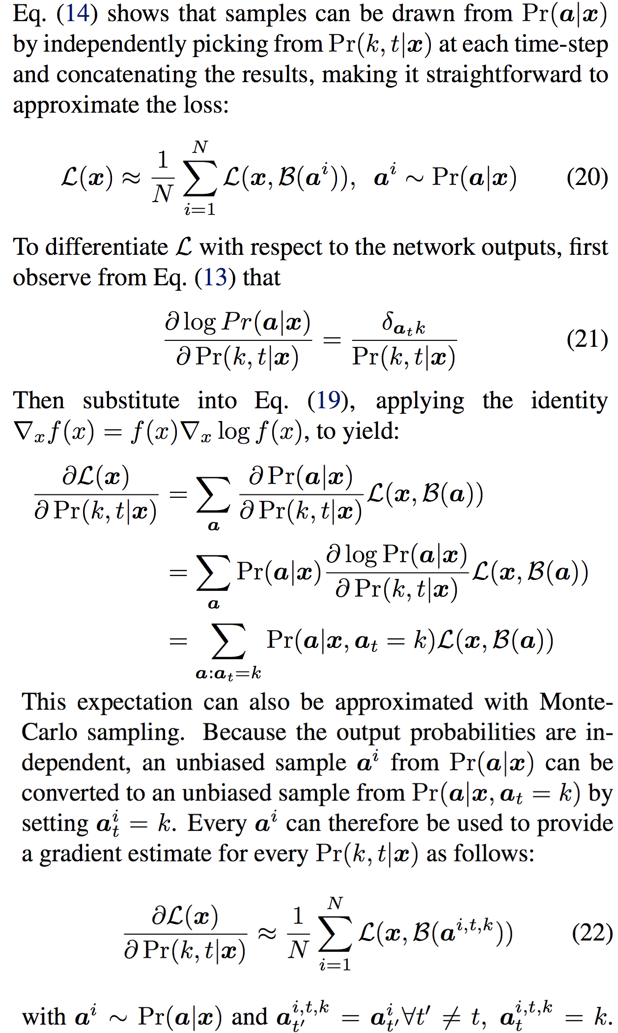
  Given input sequence $x$, the distribution $P(y\vert x)$ over transcriptions sequences $y$ defined by CTC, and a real-valued transcription loss function $\mathcal{L}(x, y)$, the expected transcription loss $\mathcal{L}(x)$ is defined:
  $$\begin{align} \mathcal{L}(x) &= \sum_y P(y \vert x)\mathcal{L}(x,y) \\ &= \sum_y \sum_{a \in \mathcal{B}^{-1}(y)} P(a \vert x)\mathcal{L}(x,y) \\ &= \sum_a P(a \vert x)\mathcal{L}(x,\mathcal{B}(a)) \end{align}$$
Algorithm:
Issues/The Bottleneck:
Results:
- WSJC ( WER):
  - Standard: $27.3\%$
  - w/Lexicon of allowed words: $21.9\%$
  - Trigram LM: $8.2\%$
  - w/Baseline system: $6.7\%$

Attention-Based Models for Speech Recognition

Introduction:

This paper introduces and extends the attention mechanism with features needed for ASR. It adds location-awareness to the attention mechanism to add robustness against different lengths of utterances.
Motivation:

Learning to recognize speech can be viewed as learning to generate a sequence (transcription) given another sequence (speech).
From this perspective it is similar to machine translation and handwriting synthesis tasks, for which attention-based methods have been found suitable.

How ASR differs:
Compared to Machine Translation, speech recognition differs by requesting much longer input sequences which introduces a challenge of distinguishing similar speech fragments in a single utterance.

thousands of frames instead of dozens of words

It is different from Handwriting Synthesis, since the input sequence is much noisier and does not have a clear structure.
Structure:
- Input: $x=(x_1, \ldots, x_{L'})$ is a sequence of feature vectors
  - Each feature vector is extracted from a small overlapping window of audio frames
- Output: $y$ a sequence of phonemes
Strategy:

The goal of this paper is a system, that uses attention-mechanism with location awareness, whose performance is comparable to that of the conventional approaches.
- For each generated phoneme, an attention mechanism selects or weighs the signals produced by a trained feature extraction mechanism at potentially all of the time steps in the input sequence (speech frames).
- The weighted feature vector then helps to condition the generation of the next element of the output sequence.
- Since the utterances in this dataset are rather short (mostly under 5 seconds), we measure the ability of the considered models in recognizing much longer utterances which were created by artificially concatenating the existing utterances.
Solves:
- Problem:
  The attention-based model proposed for NMT demonstrates vulnerability to the issue of similar speech fragments with longer, concatenated utterances.
  The paper argues that this model adapted to track the absolute location in the input sequence of the content it is recognizing, a strategy feasible for short utterances from the original test set but inherently unscalable.
- Solution:
  The attention-mechanism is modified to take into account the location of the focus from the previous step and the features of the input sequence by adding as inputs to the attention mechanism auxiliary Convolutional Features which are extracted by convolving the attention weights from the previous step with trainable filters.
Key Insights:
- Introduces attention-mechanism to ASR
- The attention-mechanism is modified to take into account:
  - location of the focus from the previous step
  - features of the input sequence
- Proposes a generic method of adding location awareness to the attention mechanism
- Introduce a modification of the attention mechanism to avoid concentrating the attention on a single frame
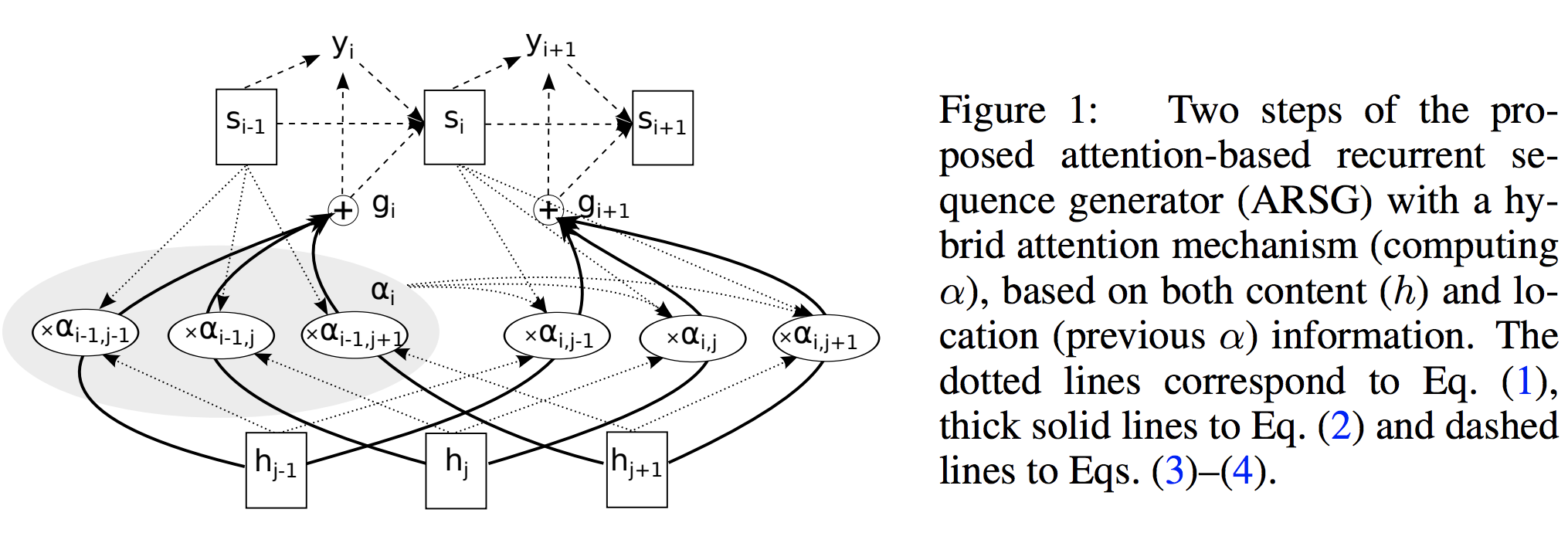
Attention-based Recurrent Sequence Generator (ARSG):

is a recurrent neural network that stochastically generates an output sequence $(y_1, \ldots, y_T)$ from an input $x$.
In practice, $x$ is often processed by an encoder which outputs a sequential input representation $h = (h_1, \ldots, h_L)$ more suitable for the attention mechanism to work with.

The Encoder: a deep bidirectional recurrent network.
It forms a sequential representation h of length $L = L'$.
Structure:
- Input: $x = (x_1, \ldots, x_{L'})$ is a sequence of feature vectors
  
  Each feature vector is extracted from a small overlapping window of audio frames.
- Output: $y$ is a sequence of phonemes
Strategy:
At the $i$-th step an ARSG generates an output $y_i$ by focusing on the relevant elements of $h$:

\[\begin{align} \alpha_i &= \text{Attend}(s_{i-1}, \alpha _{i-1}), h) & (1) \\ g_i &= \sum_{j=1}^L \alpha_{i,j} h_j & (2) // y_i &\sim \text{Generate}(s_{i-1}, g_i) & (3) \end{align}\]

where $s_{i−1}$ is the $(i − 1)$-th state of the recurrent neural network to which we refer as the generator, $\alpha_i \in \mathbb{R}^L$ is a vector of the attention weights, also often called the alignment; and $g_i$ is the glimpse.
The step is completed by computing a new generator state:

\[s_i = \text{Recurrency}(s_{i-1}, g_i, y_i)\]

where the Recurrency is an RNN.
Attention-mechanism Types and Speech Recognition:
Types of Attention:
- (Generic) Hybrid Attention: $\alpha_i = \text{Attend}(s_{i-1}, \alpha_{i-1}, h)$
- Content-based Attention: $\alpha_i = \text{Attend}(s_{i-1}, h)$
  In this case, Attend is often implemented by scoring each element in h separately and normalizing the scores:
  $e_{i,j} = \text{Score}(s_{i-1}, h_j) \\$ $\alpha_{i,j} = \dfrac{\text{exp} (e_{i,j}) }{\sum_{j=1}^L \text{exp}(e_{i,j})}$
  - Limitations:
    The main limitation of such scheme is that identical or very similar elements of $h$ are scored equally regardless of their position in the sequence.
    Often this issue is partially alleviated by an encoder such as e.g. a BiRNN or a deep convolutional network that encode contextual information into every element of h . However, capacity of h elements is always limited, and thus disambiguation by context is only possible to a limited extent.
- Location-based Attention: $\alpha_i = \text{Attend}(s_{i-1}, \alpha_{i-1})$
  a location-based attention mechanism computes the alignment from the generator state and the previous alignment only.
  - Limitations:
    the model would have to predict the distance between consequent phonemes using $s_{i−1}$ only, which we expect to be hard due to large variance of this quantity.
Thus, we conclude that the Hybrid Attention mechanism is a suitable candidate.
Ideally, we need an attention model that uses the previous alignment $\alpha_{i-1}$ to select a short list of elements from $h$, from which the content-based attention, will select the relevant ones without confusion.
Preparing the Data (Pre-Processing):

The paper uses spectrograms as a minimal preprocessing scheme.
Architecture:
Start with the ARSG-based model:
- Encoder: is a Bi-RNN
$$e_{i,j} = w^T \tanh (Ws_{i-1} + Vh_j + b)$$
- Attention: Content-Based Attention extended for location awareness
  $$e_{i,j} = w^T \tanh (Ws_{i-1} + Vh_j + Uf_{i,j} + b)$$
Extending the Attention Mechanism:
Content-Based Attention extended for location awareness by making it take into account the alignment produced at the previous step.
- First, we extract $k$ vectors $f_{i,j} \in \mathbb{R}^k$ for every position $j$ of the previous alignment $\alpha_{i−1}$ by convolving it with a matrix $F \in \mathbb{R}^{k\times r}$:
  $$f_i = F * \alpha_{i-1}$$
- These additional vectors $f_{i,j} are then used by the scoring mechanism$e_{i,j}$$:
  $$e_{i,j} = w^T \tanh (Ws_{i-1} + Vh_j + Uf_{i,j} + b)$$
Algorithm:
Issues/The Bottleneck:
Asynchronous:

Attention Is All You Need

Introduction:
This paper introduces the Transformer network architecture.
The model relies completely on Attention and disregards recurrence/convolutions completely.
Motivation:
Motivation for Dropping:
- Recurrent Connections:
  - Complex
  - Tricky to Train and Regularize
  - Capturing long-term dependencies is limited and hard to parallelize
  - Sequence-aligned states in RNN are wasteful.
  - Hard to model hierarchical-like domains such as languages.
- Convolutional Connections:
  - Convolutional approaches are sometimes effective (more on this)
  - But they tend to be memory-intensive.
  - Path length between positions can be logarithmic when using dilated convolutions; and Left-padding (for text). (autoregressive CNNs WaveNet, ByteNET)
    - However, Long-distance dependencies require many layers.
  - Modeling long-range dependencies with CNNs requires either:
    - Many Layers: likely making training harder
    - Large Kernels: at large parameter/computational cost
Motivation for Transformer:
It gives us the shortest possible path through the network between any two input-output locations.

Motivation in NLP:
The following quote:
“You can’t cram the meaning of a whole %&!$# sentence into a single $&!#* vector!” - ACL 2014
Idea:
Why not use Attention for Representations?
- Self-Attention: You try to represent (re-express) yourself (the word_i) as a weighted combination of your entire neighborhood
- FFN Layers: they compute new features for the representations from the attention weighted combination
- Residual Connections: Residuals carry/propagate positional information about the inputs to higher layers, among other info.
- Attention-Layer:
  - Think of as a feature detector.
From Attention to Self-Attention:
The Encoder-Decoder Architecture:
For a fixed target output, $t_j$, all hidden state source inputs are taken into account to compute the cosine similarity with the source inputs $s_i$, to generate the $\theta_i$’s (attention weights) for every source input $s_i$.
Strategy:
The idea here is to learn a context vector (say $U$), which gives us global level information on all the inputs and tells us about the most important information.
E.g. This could be done by taking a cosine similarity of this context vector $U$ w.r.t the input hidden states from the fully connected layer. We do this for each input $x_i$ and thus obtain a $\theta_i$ (attention weights).

The Goal(s):
- Parallelization of Seq2Seq: RNN/CNN handle sequences word-by-word sequentially which is an obstacle to parallelize.
  Transformer achieves parallelization by replacing recurrence with attention and encoding the symbol position in the sequence.
  This, in turn, leads to a significantly shorter training time.
- Reduce sequential computation: Constant $\mathcal{O}(1)$ number of operations to learn dependency between two symbols independently of their position/distance in sequence.
The Transformer reduces the number of sequential operations to relate two symbols from input/output sequences to a constant $\mathcal{O}(1)$ number of operations.
It achieves this with the multi-head attention mechanism that allows it to model dependencies regardless of their distance in input or output sentence (by counteracting reduced effective resolution due to averaging the attention-weighted positions).
Architecture:

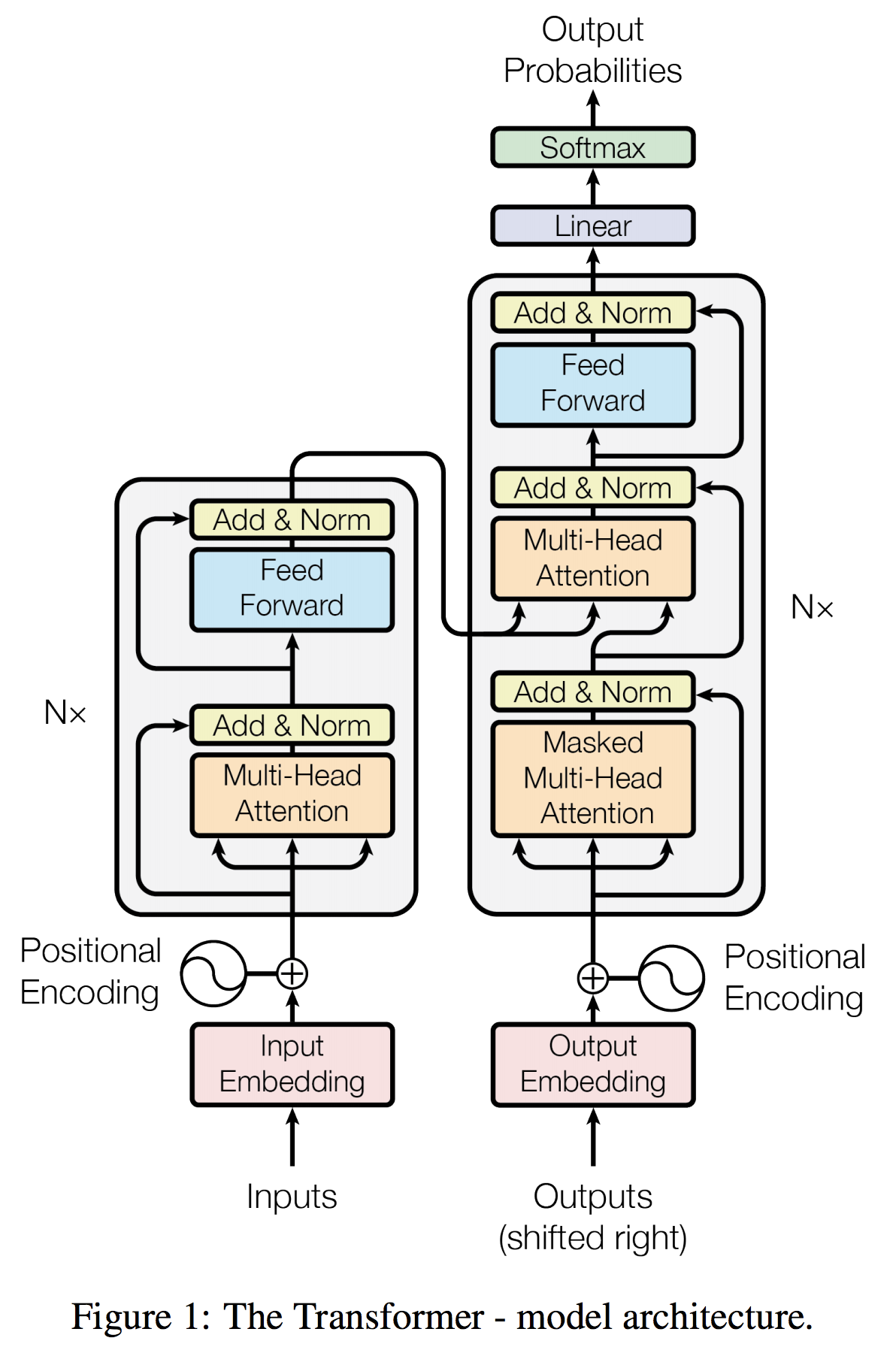
The Transformer follows a Encoder-Decoder architecture using stacked self-attention and point-wise, fully connected layers for both the encoder and decoder, shown in the left and right halves of Figure 1, respectively:

Encoder:
The encoder is composed of a stack of $N = 6$ identical layers. Each layer has two sub-layers. The first is a multi-head self-attention mechanism, and the second is a simple, positionwise fully connected feed-forward network. We employ a residual connection around each of the two sub-layers, followed by layer normalization. That is, the output of each sub-layer is $\text{LayerNorm}(x + \text{Sublayer}(x))$, where $\text{Sublayer}(x)$ is the function implemented by the sub-layer itself. To facilitate these residual connections, all sub-layers in the model, as well as the embedding layers, produce outputs of dimension $d_{\text{model}} = 512$.

Decoder:
The decoder is also composed of a stack of $N = 6$ identical layers. In addition to the two sub-layers in each encoder layer, the decoder inserts a third sub-layer, which performs multi-head attention over the output of the encoder stack. Similar to the encoder, we employ residual connections around each of the sub-layers, followed by layer normalization. We also modify the self-attention sub-layer in the decoder stack to prevent positions from attending to subsequent positions. This masking, combined with fact that the output embeddings are offset by one position, ensures that the predictions for position $i$ can depend only on the known outputs at positions less than $i$.

The Encoder maps an input sequence of symbol representations $(x_1, \ldots, x_n)$ to a sequence of continuous representations $z = (z_1, ..., z_n)$.
Given $z$, the decoder then generates an output sequence $(y_1, ..., y_m)$ of symbols one element at a time. At each step the model is auto-regressive, consuming the previously generated symbols as additional input when generating the next.
The Model - Attention:
Formulation: Standard attention with queries and key, value pairs.
- Scaled Dot-Product Attention:
  
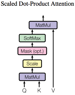
  Given: (1) Queries $\vec{q} \in \mathbb{R}^{d_k}$ (2) Keys $\vec{k} \in \mathbb{R}^{d_k}$ (3) Values $\vec{v} \in \mathbb{R}^{d_v}$
  Computes the dot products of the queries with all keys; scales each by $\sqrt{d_k}$; and normalizes with a softmax to obtain the weights $\theta_i$s on the values.
  For a given query vector $\vec{q} = \vec{q}_j$ for some $j$:
  $${\displaystyle \vec{o} = \sum_{i=0}^{d_k} \text{softmax} (\dfrac{\vec{q}^T \: \vec{k}_i}{\sqrt{d_k}}) \vec{v}_i = \sum_{i=0}^{d_k} \theta_i \vec{v}_i}$$
  
  In practice, we compute the attention function on a set of queries simultaneously, in matrix form (stacked row-wise):
  
  $${\displaystyle \text{Attention}(Q, K, V) = O = \text{softmax} (\dfrac{QK^T}{\sqrt{d_k}}) V } \tag{1}$$
  
  Motivation: We suspect that for large values of $d_k$, the dot products grow large in magnitude, pushing the softmax function into regions where it has extremely small gradients. To counteract this effect, we scale the dot products by $\sqrt{\dfrac{1}{d_k}}$.
- Multi-Head Attention:
  
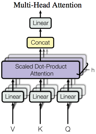
  Instead of performing a single attention function with $d_{\text{model}}$-dimensional keys, values and queries; linearly project the queries, keys and values $h$ times with different, learned linear projections to $d_k, d_k$ and $d_v$ dimensions, respectively. Then, attend (apply $\text{Attention}$ function) on each of the projected versions, in parallel, yielding $d_v$-dimensional output values. The final values are obtained by concatenating and projecting the $d_v$-dimensional output values from each of the attention-heads.
  $$\begin{aligned} \text {MultiHead}(Q, K, V) &=\text {Concat}\left(\text {head}_ {1}, \ldots, \text {head}_ {h}\right) W^{O} \\ \text { where head}_ {i} &=\text {Attention}\left(Q W_{i}^{Q}, K W_{i}^{K}, V W_{i}^{V}\right) \end{aligned}$$
  
  Where the projections are parameter matrices $W_{i}^{Q} \in \mathbb{R}^{d_{\text {model}} \times d_{k}}, W_{i}^{K} \in$ $\mathbb{R}^{d_{\text {model}} \times d_{k}},$ $W_{i}^{V} \in \mathbb{R}^{d_{\text {model}} \times d_{v}}$ and $W^O \in \mathbb{R}^{hd_v \times d_{\text {model}}}$.
  This paper choses $h = 8$ parallel attention layers/heads.
  For each, they use $d_k=d_v=d_{\text{model}}/h = 64$.
  The reduced dimensionality of each head, allows the total computation cost to be similar to that of a single head w/ full dimensionality.
  
  Motivation: Multi-head attention allows the model to jointly attend to information from different representation subspaces at different positions. With a single attention head, averaging inhibits this.
Applications of Attention in the Model:
The Transformer uses multi-head attention in three different ways:
- Encode-Decoder Attention Layer (standard layer):
  - The queries come from: the previous decoder layer
  - The memory keys and values come from: the output of the encoder
  This allows every position in the decoder to attend over all positions in the input sequence.
- Encoder Self-Attention:
  The encoder contains self-attention layers.
  - Both, The queries, and keys and values, come from: the encoders output of previous layer
  Each position in the encoder can attend to all positions in the previous layer of the encoder.
- Decoder Self-Attention:
  The decoder, also, contains self-attention layers.
  - Both, The queries, and keys and values, come from: the decoders output of previous layer
  However, self-attention layers in the decoder allow each position in the decoder to attend to all positions in the decoder up to, and including, that position. Since, we need to prevent leftward information flow in the decoder to preserve the auto-regressive property.
  This is implemented inside of scaled dot-product attention by masking out (setting to $-\infty$ ) all values in the input of the softmax which correspond to illegal connections.
The Model - Position-wise Feed-Forward Network (FFN):
In addition to attention sub-layers, each of the layers in our encoder and decoder contains a fully connected feed-forward network, which is applied to each position separately and identically.
It consists of two linear transformations with a ReLU activation in between:
$$\text{FFN}(x) = \max(0, xW_1 + b_1)W_2 + b_2 \tag{2}$$

While the linear transformations are the same across different positions, they use different parameters from layer to layer.

Equivalently, we can describe this as, two convolutions with kernel-size $= 1$

Dimensional Analysis:
- Input/Output: $\in \mathbb{R}^{d_\text{model} = 512}$
- Inner-Layer: $\in \mathbb{R}^{d_{ff} = 2048}$
The Model - Embeddings and Softmax:
Use learned embeddings to convert the input tokens and output tokens to vectors $\in \mathbb{R}^d_{\text{model}}$.
Use the usual learned linear transformation and softmax to convert decoder output to predicted next-token probabilities.

The model shares the same weight matrix between the two embedding layers and the pre-softmax linear transformation.
In the embedding layers, multiply those weights by $\sqrt{d_{\text{model}}}$.
The Model - Positional Encoding:
Motivation:
Since the model contains no recurrence and no convolution, in order for the model to make use of the order of the sequence, we must inject some information about the relative or absolute position of the tokens in the sequence.

Positional Encoding:
A way to add positional information to an embedding.
There are many choices of positional encodings, learned and fixed. [Gehring et al. 2017]
The positional encodings have the same dimension $d_{\text{model}}$ as the embeddings, so that the two can be summed.

Approach:
Add “positional encodings” to the input embeddings at the bottoms of the encoder and decoder stacks.
Use sine and cosine functions of different frequencies:

$$ \begin{aligned} P E_{(\text{pos}, 2 i)} &=\sin \left(\text{pos} / 10000^{2 i / d_{\mathrm{model}}}\right) \\ P E_{(\text{pos}, 2 i+1)} &=\cos \left(\text{pos}/ 10000^{2 i / d_{\mathrm{model}}}\right) \end{aligned} $$

where $\text{pos}$ is the position and $i$ is the dimension.
That is, each dimension of the positional encoding corresponds to a sinusoid. The wavelengths form a geometric progression from $2\pi$ to $10000 \cdot 2\pi$.

Motivation:
We chose this function because we hypothesized it would allow the model to easily learn to attend by relative positions, since for any fixed offset $k$, $PE_{pos + k}$ can be represented as a linear function of $P E_{pos}$.

Sinusoidal VS Learned: We chose the sinusoidal version (instead of learned positional embeddings, with similar results) because it may allow the model to extrapolate to sequence lengths longer than the ones encountered during training.
Training Tips & Tricks:
- Layer Normalization: Help ensure that layers remain in reasonable range
- Specialized Training Schedule: Adjust default learning rate of the Adam optimizer
- Label Smoothing: Insert some uncertainty in the training process
- Masking (for decoder attention): for Efficient Training using matrix-operations
Why Self-Attention? (as opposed to Conv/Recur. layers):

Total Computational Complexity per Layer:
- Self-Attention layers are faster than recurrent layers when the sequence length $n$ is smaller than the representation dimensionality $d$.
  
  Which is most often the case with sentence representations used by state-of-the-art models in machine translations, such as word-piece and byte-pair representations.
- To improve computational performance for tasks involving very long sequences, self-attention could be restricted to considering only a neighborhood of size $r$ in the input sequence centered around the respective output position.
  This would increase the maximum path length to $\mathcal{O}(n/r)$.
Parallelizable Computations: (measured by the minimum number of sequential ops required)
Self-Attention layers connect all positions with a constant number of sequentially executed operations, whereas a recurrent layer requires $\mathcal{O}(n)$ sequential operations.

Path Length between Positions: (Long-Range Dependencies)
- Convolutional Layers: A single convolutional layer with kernel width $k < n$ does not connect all pairs of input and output positions.
  Doing so requires:
  - Contiguous Kernels (valid): a stack of $\mathcal{O}(n/k)$ convolutional layers
  - Dilated Kernels: $\mathcal{O}(\log_k(n))$
    increasing the length of the longest paths between any two positions in the network.
  - Separable Kernels: decrease the complexity considerably, to $\mathcal{O}\left(k \cdot n \cdot d+n \cdot d^{2}\right)$
  Convolutional layers are generally more expensive than recurrent layers, by a factor of $k$.
- Self-Attention:
  Even with $k = n$, the complexity of a separable convolution is equal to the combination of a self-attention layer and a point-wise feed-forward layer, the approach taken in this model.
Interpretability:
As side benefit, self-attention could yield more interpretable models.
Not only do individual attention heads clearly learn to perform different tasks, many appear to exhibit behavior related to the syntactic and semantic structure of the sentences.
Results:
- Attention Types:
  For small values of $d_k$ the two mechanisms perform similarly, additive attention outperforms dot product attention without scaling for larger values of $d_k$.
- Positional Encodings:
  We also experimented with using learned positional embeddings instead, and found that the two versions produced nearly identical results.

Deep Learning
Research Papers

Table of Contents

Sequence to Sequence Learning with Neural Network

Towards End-to-End Speech Recognition with Recurrent Neural Networks

Attention-Based Models for Speech Recognition

Attention Is All You Need

Deep Learning Research Papers

Table of Contents

Sequence to Sequence Learning with Neural Network

Towards End-to-End Speech Recognition with Recurrent Neural Networks

Attention-Based Models for Speech Recognition

Attention Is All You Need

Deep Learning
Research Papers