Machine Translation

1. Methods:

   • Methods are statistical
   • Uses parallel corpora

2. Traditional MT:

   Traditional MT was very complex and included multiple disciplines coming in together.
   The systems included many independent parts and required a lot of human engineering and experts.
   The systems also scaled very poorly as the search problem was essentially exponential.

3. Statistical Machine Translation Systems:

   • Input:
     • Source Language: \(f\)
     • Target Language: \(e\)
   • The Probabilistic Formulation:

   \[\hat{e} = \mathrm{arg\,min}_e \: p(e \vert f) = \mathrm{arg\,min}_e \: p(f \vert e) p(e)\]

   • The Translation Model \(p(f \vert e)\): trained on parallel corpus
   • The Language Model \(p(e)\): trained on English only corpus

     Abundant and free!

   

4. Deep Learning Naive Approach:

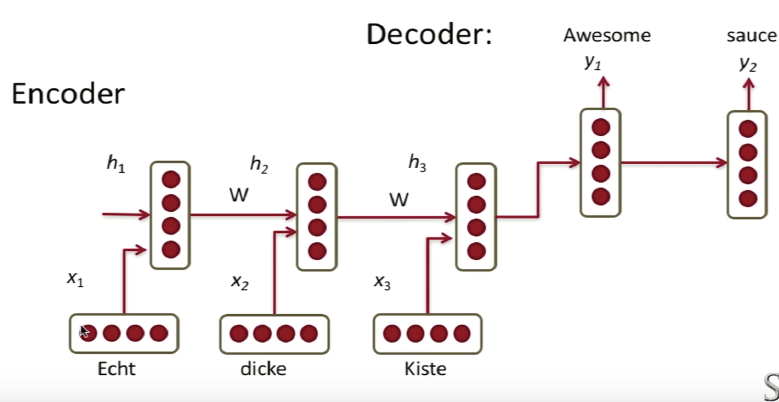
   One way we can learn to translate is to learn to translate directly with an RNN.

   

   • The Model:
     • Encoder :
       \(h_t = \phi(h_{t-1}, x_t) = f(W^{(hh)}h_{t-1} + W^{(hx)}x_t)\)
     • Decoder :
       \(\begin{align} h_t & = \phi(h_{t-1}) = f(W^{(hh)}h_{t-1}) \\ y_t & = \text{softmax}(W^{(S)}h_t) \end{align}\)
     • Error :
       \(\displaystyle{\max_\theta \frac{1}{N} \sum_{n=1}^N \log p_\theta(y^{(n)}\vert x^{(n)})}\)

       Cross Entropy Error.

     • Goal :
       Minimize the Cross Entropy Error for all target words conditioned on source words

   • Drawbacks:
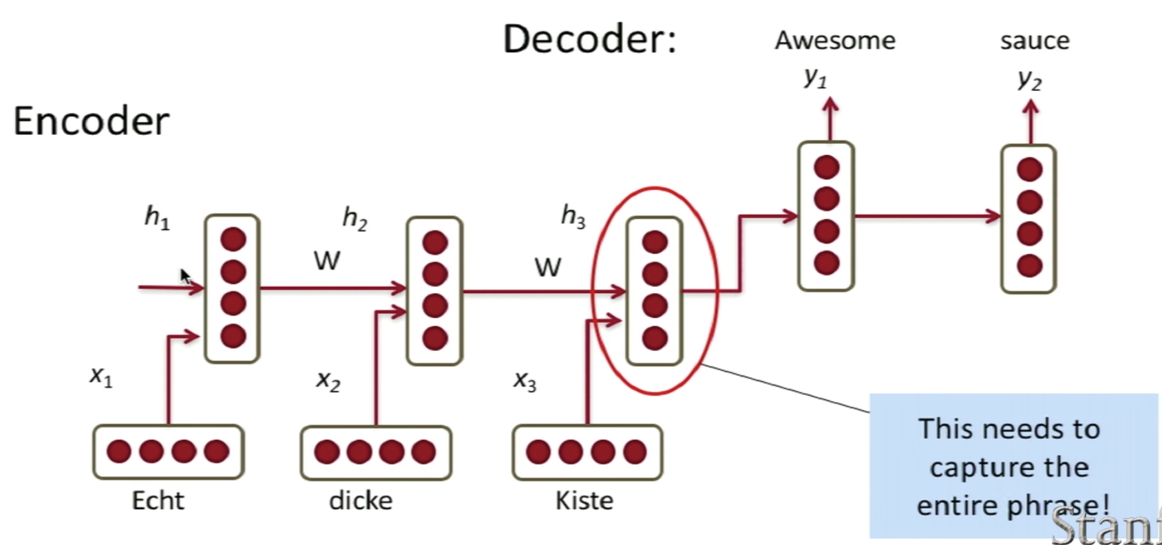
     The problem of this approach lies in the fact that the last hidden layer needs to capture the entire sentence to be translated.
     However, since we know that the RNN Gradient basically vanishes as the length of the sequence increases, the last hidden layer is usually only capable of capturing upto ~5 words.

   

5. Naive RNN Translation Model Extension:

   1. Train Different RNN weights for encoding and decoding
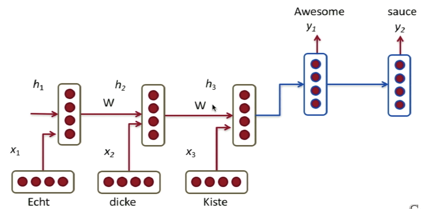
   2. Compute every hidden state in the decoder from the following concatenated vectors :
      • Previous hidden state (standard)
      • Last hidden vector of encoder \(c=h_T\)
      • Previous predicted output word \(y_{t-1}\).
        \(\implies h_{D, t} = \phi_D(h_{t-1}, c, y_{t-1})\)

        NOTE: Each input of \(\phi\) has its own linear transformation matrix.

   3. Train stacked/deep RNNs with multiple layers.
   4. Potentially train Bidirectional Encoder
   5. Train input sequence in reverser order for simpler optimization problem:
      Instead of \(A\:B\:C \rightarrow X\:Y\) train with \(C\:B\:A \rightarrow X\:Y\)
   6. Better Units (Main Improvement):
      • Use more complex hidden unit computation in recurrence
      • Use GRUs (Cho et al. 2014)
      • Main Ideas:
        • Keep around memories to capture long distance dependencies
        • Allow error messages to flow at different strengths depending on the inputs

GRUs

1. Gated Recurrent Units:

   Gated Recurrent Units (GRUs) are a class of modified (Gated) RNNs that allow them to combat the vanishing gradient problem by allowing them to capture more information/long range connections about the past (memory) and decide how strong each signal is.

2. Main Idea:

   Unlike standard RNNs which compute the hidden layer at the next time step directly first, GRUs computes two additional layers (gates):

   Each with different weights

   • Update Gate:

   \[z_t = \sigma(W^{(z)}x_t + U^{(z)}h_{t-1})\]

   • Reset Gate:

   \[r_t = \sigma(W^{(r)}x_t + U^{(r)}h_{t-1})\]

   The Update Gate and Reset Gate computed, allow us to more directly influence/manipulate what information do we care about (and want to store/keep) and what content we can ignore.
   We can view the actions of these gates from their respecting equations as:

   • New Memory Content:
     at each hidden layer at a given time step, we compute some new memory content,
     if the reset gate \(= ~0\), then this ignores previous memory, and only stores the new word information.

   \[\tilde{h}_t = \tanh(Wx_t + r_t \odot Uh_{t-1})\]

   • Final Memory:
     the actual memory at a time step \(t\), combines the Current and Previous time steps,
     if the update gate \(= ~0\), then this, again, ignores the newly computed memory content, and keeps the old memory it possessed.

   \[h_t = z_t \odot h_{t-1} + (1-z_t) \odot \tilde{h}_t\]

Long Short-Term Memory

1. LSTM:

   The Long Short-Term Memory (LSTM) Network is a special case of the Recurrent Neural Network (RNN) that uses special gated units (a.k.a LSTM units) as building blocks for the layers of the RNN.

2. Architecture:

   The LSTM, usually, has four gates:

   • Input Gate: The input gate determines how much does the current input vector (current cell) matters

   \[i_t = \sigma(W^{(i)}x_t + U^{(i)}h_{t-1})\]

   • Forget Gate: Determines how much of the past memory, that we have kept, is still needed

   \[i_t = \sigma(W^{(i)}x_t + U^{(i)}h_{t-1})\]

   • Output Gate: Determines how much of the current cell matters for our current prediction (i.e. passed to the sigmoid)

   \[i_t = \sigma(W^{(i)}x_t + U^{(i)}h_{t-1})\]

   • Memory Cell: The memory cell is the cell that contains the short-term memory collected from each input

   \[\begin{align} \tilde{c}_t & = \tanh(W^{(c)}x_t + U^{(c)}h_{t-1}) & \text{New Memory} \\ c_t & = f_t \odot c_{t-1} + i_t \odot \tilde{c}_t & \text{Final Memory} \end{align}\]

   The Final Hidden State is calculated as follows:

   \[h_t = o_t \odot \sigma(c_t)\]

3. Properties:

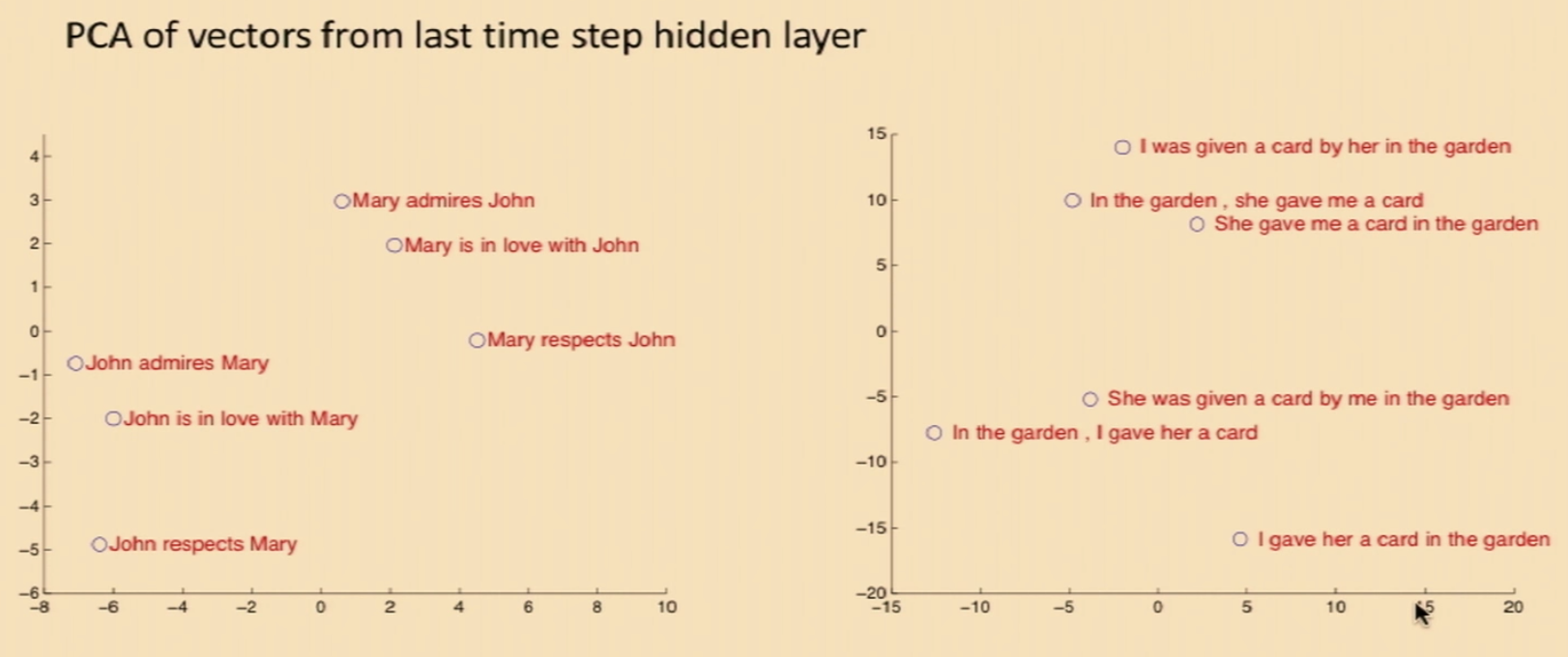
   • Syntactic Invariance:
     When one projects down the vectors from the last time step hidden layer (with PCA), one can observe the spatial localization of syntacticly-similar sentences
     

Neural Machine Translation (NMT)

1. NMT:

   NMT is an approach to machine translation that uses a large artificial neural network to predict the likelihood of a sequence of words, typically modeling entire sentences in a single integrated model.

2. Architecture:

   The approach uses an Encoder-Decoder architecture.

   

   NMT models can be seen as a special case of language models.
   In other words, they can be seen as Conditional Recurrent Language Model; a language model that has been conditioned on the calculated encoded vector representation of the sentence.

3. Modern Sequence Models for NMT:

4. Issues of NMT:

   • Predicting Unseen Words:
     The NMT model is very vulnerable when presented with a word that it has never seen during training (e.g. a new name).
     In-fact, the model might not even be able to place the (translated) unseen word correctly in the (translated) sentence.
   • Solution:
     • A possible solution is to apply character-based translation, instead of word-based, however, this approach makes for very long sequences and the computation becomes infeasible.
     • The (current) proposed approach is to use a Mixture Model of Softmax and Pointers

       Pointer-sentinel Model

5. The Big Wins of NMT:

   1. End-to-End Training: All parameters are simultaneously optimized to minimize a loss function on the networks output
   2. Distributed Representations Share Strength: Better exploitation of word and phrase similarities
   3. Better Exploitation of Context: NMT can use a much bigger context - both source and partial target text - to translate more accurately
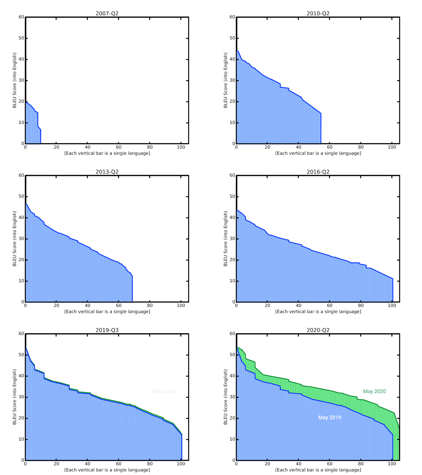
   4. More Fluent Text Generation: Deep Learning text generation is much higher quality

   Progress in Google Translate based on a one sentence test set from C. Manning

   Google Translate BLEU Score Progression

6. (GNMT) Google’s Multilingual Neural Machine Translation System - Zero shot Translation:

   • Multilingual NMT Approaches:

   

   • Google’s Approach:
     Add an Artificial Token at the beginning of the input sentence to indicate the target language.

Notes:

• Evaluation Metrics: BLEU Score: or Bilingual Evaluation Understudy Score

  The second most popular score is METEOR: which has an emphasis on recall and precision.