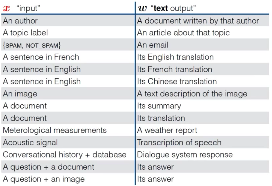
Table of Contents
Language Modeling and RNNS I (Oxford)
Note: 25:00 (important problem not captured w/ newer models about smoothing and language distribution as Heaps law)
Introduction to and History of Language Models
-
Language Models:
A Language Model is a statistical model that computes a probability distribution over sequences of words.It is a time-series prediction problem in which we must be very careful to train on the past and test on the future.
-
- Applications:
-
- Machine Translation (MT):
- Word Ordering:
p(“the cat is small”) > p(“small the cat is”) - Word Choice:
p(“walking home after school”) > p(“walking house after school”)
- Word Ordering:
- Speech Recognition:
- Word Disambiguation:
p(“The listeners recognize speech”) > p(“The listeners wreck a nice beach”)
- Word Disambiguation:
- Information Retrieval:
- Used in query likelihood model
- Machine Translation (MT):
- Traditional Language Models:
- Most language models employ the chain rule to decompose the joint probability into a sequence of conditional probabilities:
$$\begin{array}{c}{P\left(w_{1}, w_{2}, w_{3}, \ldots, w_{N}\right)=} \\ {P\left(w_{1}\right) P\left(w_{2} | w_{1}\right) P\left(w_{3} | w_{1}, w_{2}\right) \times \ldots \times P\left(w_{N} | w_{1}, w_{2}, \ldots w_{N-1}\right)}\end{array}$$
Note that this decomposition is exact and allows us to model complex joint distributions by learning conditional distributions over the next word \((w_n)\) given the history of words observed \(\left(w_{1}, \dots, w_{n-1}\right)\).
Thus, the Goal of the LM-Task is to find good conditional distributions that we can multiply to get the Joint Distribution.Allows you to predict the first word, then the second word given the first word, then the third given the first two, etc..
- The Probability is usually conditioned on window of \(n\) previous words
- An incorrect but necessary Markovian assumption:
$$P(w_1, \ldots, w_m) = \prod_{i=1}^m P(w_i | w_1, \ldots, w_{i-1}) \approx \prod_{i=1}^m P(w_i | w_{i-(n-1)}, \ldots, w_{i-1})$$
- Only previous history matters
- Limited Memory: only last \(n-1\) words are included in history
E.g. \(2-\)gram LM (only looks at the previous word):
$$\begin{aligned} p\left(w_{1}, w_{2}, w_{3},\right.& \ldots &, w_{n} ) \\ &=p\left(w_{1}\right) p\left(w_{2} | w_{1}\right) p\left(w_{3} | w_{1}, w_{2}\right) \times \ldots \\ & \times p\left(w_{n} | w_{1}, w_{2}, \ldots w_{n-1}\right) \\ & \approx p\left(w_{1}\right) p\left(w_{2} | w_{1}\right) p\left(w_{3} | w_{2}\right) \times \ldots \times p\left(w_{n} | w_{n-1}\right) \end{aligned}$$
The conditioning context, \(w_{i-1}\), is called the history.
- An incorrect but necessary Markovian assumption:
- The MLE estimate for probabilities, compute for
- Bi-grams:
$$P(w_2 \| w_1) = \dfrac{\text{count}(w_1, w_2)}{\text{count}(w_1)}$$
- Tri-grams:
$$P(w_3 \| w_1, w_2) = \dfrac{\text{count}(w_1, w_2, w_3)}{\text{count}(w_1, w_2)}$$
- Bi-grams:
- Most language models employ the chain rule to decompose the joint probability into a sequence of conditional probabilities:
- Issues with the Traditional Approaches:
To improve performance we need to:- Keep higher n-gram counts
- Use Smoothing
- Use Backoff (trying n-gram, (n-1)-gram, (n-2)-grams, ect.)
When? If you never saw a 3-gram b4, try 2-gram, 1-gram etc.
However, - There are A LOT of n-grams
- \(\implies\) Gigantic RAM requirements
- NLP Tasks as LM Tasks:
Much of Natural Language Processing can be structured as (conditional) Language Modeling:- Translation:
$$p_{\mathrm{LM}}(\text { Les chiens aiment les os }\| \| \text { Dogs love bones) }$$
- QA:
$$p_{\mathrm{LM}}(\text { What do dogs love? }\| \| \text { bones } . | \beta)$$
- Dialog:
$$p_{\mathrm{LM}}(\text { How are you? }\| \| \text { Fine thanks. And you? } | \beta)$$
where \(\| \|\) means “concatenation”, and \(\beta\) is an observed data (e.g. news article) to be conditioned on.
- Translation:
-
Analyzing the LM Tasks:
The simple objective of modeling the next word given observed history contains much of the complexity of natural language understanding (NLU) (e.g. reasoning, intelligence, etc.).Consider predicting the extension of the utterance:
$$p(\cdot | \text { There she built a) }$$
The distribution of what word to predict right now is quite flat; you dont know where “there” is, you dont know who “she” is, you dont know what she would want to “build”.
However, With more context we are able to use our knowledge of both language and the world to heavily constrain the distribution over the next word.
$$p(\cdot | \color{red} {\text { Alice }} \text {went to the} \color{blue} {\text { beach. } } \color{blue} {\text {There}} \color{red} {\text { she}} \text { built a})$$
At this point your distributions getting very peaked about what could come next and the reason is because you understand language you understand that in the second utterance “she” is “Alice” and “There” is “Beach” so you’ve resolved those Co references and you can do that because you understand the syntactic structure of the first utterance; you understand we have a subject and object, where the verb phrase is, all of these things you do automatically and then, using the semantics that “at a beach you build things like sandcastles or boats” and so you can constrict your distribution.
If we can get a automatically trained machine to do that then we’ve come a long way to solving AI.
“The diversity of tasks the model is able to perform in a zero-shot setting suggests that high-capacity models trained to maximize the likelihood of a sufficiently varied text corpus begin to learn how to perform a surprising amount of tasks without the need for explicit supervision” - GPT 2
- Evaluating a Language Model | The Loss:
For a probabilistic model, it makes sense to evaluate how well the “learned” distribution matches the real distribution of the data (of real utterances). A good model assigns real utterances \(w_{1}^{N}\) from a language a high probability. This can be measured with Cross-Entropy:$$H\left(w_{1}^{N}\right)=-\frac{1}{N} \log _{2} p\left(w_{1}^{N}\right)$$
Why Cross-Entropy: It is a measure of how many bits are need to encode text with our model (bits you would need to represent the distribution).1
Commonly used for character-level.
Alternatively, people tend to use Perplexity:
$$\text { perplexity }\left(w_{1}^{N}\right)=2^{H\left(w_{1}^{N}\right)}$$
Why Perplexity: It is a measure of how surprised our model is on seeing each word.
If no surprise, the perplexity \(= 1\).
Commonly used for word-level.
-
Language Modeling Data:
Language modelling is a time series prediction problem in which we must be careful to train on the past and test on the future.
If the corpus is composed of articles, it is best to ensure the test data is drawn from a disjoint set of articles to the training data.Two popular data sets for language modeling evaluation are a preprocessed version of the Penn Treebank,1 and the Billion Word Corpus.2 Both are flawed:
- The PTB is very small and has been heavily processed. As such it is not representative of natural language.
- The Billion Word corpus was extracted by first randomly permuting sentences in news articles and then splitting into training and test sets. As such train and test sentences come from the same articles and overlap in time
The recently introduced WikiText datasets are a better option.
- Three Approaches to Parameterizing Language Models:
- Count-Based N-gram models: we approximate the history of observed words with just the previous \(n\) words.
They capture Multinomial distributions. - Neural N-gram models: embed the same fixed n-gram history in a continuous space and thus better capture correlations between histories.
Replace the Multinomial distributions with an FFN. - RNNs: drop the fixed n-gram history and compress the entire history in a fixed length vector, enabling long range correlations to be captured.
Replace the finite history, captured by the conditioning context \(w_{i-1}\), with an infinite history, captured by the (previous) hidden state \(h_{n-1}\) (but also \(w_{n=1})\).
- Count-Based N-gram models: we approximate the history of observed words with just the previous \(n\) words.
- Bias vs Variance in LM Approximations:
The main issue in language modeling is compressing the history (a string). This is useful beyond language modeling in classification and representation tasks.- With n-gram models we approximate the history with only the last n words
- With recurrent models (RNNs, next) we compress the unbounded history into a fixed sized vector
We can view this progression as the classic Bias vs. Variance tradeoff in ML:
- N-gram models: are biased but low variance.
No matter how much data (infinite) they will always be wrong/biased. - RNNs: decrease the bias considerably, hopefully at a small cost to variance.
Consider predicting the probability of a sentence by how many times you have seen it before. This is an unbiased estimator with (extremely) high variance.
- In the limit of infinite data, gives true distribution.
- Scaling Language Models (Large Vocabularies):
Bottleneck:
Much of the computational cost of a Neural LM is a function of the size of the vocabulary and is dominated by calculating the softmax:$$\hat{p}_{n}=\operatorname{softmax}\left(W h_{n}+b\right)$$
Solutions:
- Short-Lists: use the neural LM for the most frequent words, and a traditional n-gram LM for the rest.
While easy to implement, this nullifies the Neural LMs main advantage, i.e. generalization to rare events. - Batch local short-lists: approximate the full partition function for data instances from a segment for the data with a subset of vocabulary chosen for that segment.
- Approximate the gradient/change the objective: if we did not have to sum over the vocabulary to normalize during training, it would be much faster. It is tempting to consider maximizing likelihood by making the log partition function an independent parameter \(c\), but this leads to an ill defined objective:
$$\hat{p}_{n} \equiv \exp \left(W h_{n}+b\right) \times \exp (c)$$
What does the Softmax layer do?
The idea of the Softmax is to say: at each time step look at the word we want to predict and the whole vocab; where we try to maximize the probability of the word we want to predict and minimize the probability of ALL THE OTHER WORDS.So, The better solution is to try to approximate what the softmax does using:
- Noise Contrastive Estimation (NCE): this amounts to learning a binary classifier to distinguish data samples from \((k)\) samples from a noise distribution (a unigram is a good choice):
$$p\left(\text { Data }=1 | \hat{p}_{n}\right)=\frac{\hat{p}_{n}}{\hat{p}_{n}+k p_{\text { noise }}\left(w_{n}\right)}$$
Now parametrizing the log partition function as \(c\) does not degenerate. This is very effective for speeding up training but has no effect on testing.
- Importance Sampling (IS): similar to NCE but defines a multiclass classification problem between the true word and noise samples, with a Softmax and cross entropy loss.
- (more on) Approximating the Softmax
- Factorize the output vocabulary: the idea is to decompose the (one big) softmax into a series of softmaxes (2 in this case). We map words to a set of classes, then we, first, predict which class the word is in, and then we predict the right word from the words in that class.
One level factorization works well (Brown clustering is a good choice, frequency binning is not):$$p\left(w_{n} | \hat{p}_{n}^{\text { class }}, \hat{p}_{n}^{\text { word }}\right)=p\left(\operatorname{class}\left(w_{n}\right) | \hat{p}_{n}^{\text { class }}\right) \times p\left(w_{n} | \operatorname{class}\left(w_{n}\right), \hat{p}_ {n}^{\text { word }}\right)$$
where the function \(\text{ class}(\cdot)\) maps each word to one class. Assuming balanced classes, this gives a quadratic, \(\root{V}\) speedup.
Complexity Comparison of the different solutions:
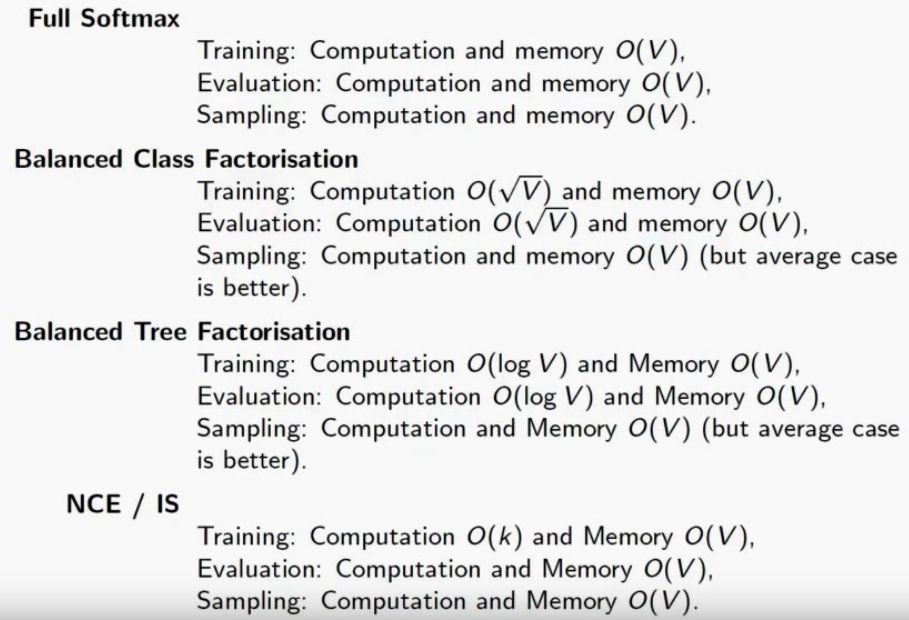
- Short-Lists: use the neural LM for the most frequent words, and a traditional n-gram LM for the rest.
-
Sub-Word Level Language Models:
Could be viewed as an alternative to changing the softmax by changing the input granularity and model text at the morpheme or character level.
This results in a much smaller softmax and no unknown words, but the downsides are longer sequences and longer dependencies; moreover, a lot of the structure in a language is in the words and we want to learn correlations amongst the words but since the model doesn’t get the words as a unit, it will have to learn what/where a is before it can learn its correlation with other sequences; which effecitely means that we made the learning problem harder and more non-linear
This, also, allows the model to capture subword structure and morphology: e.g. “disunited” <-> “disinherited” <-> “disinterested”.
Character LMs lag behind word-based models in perplexity, but are clearly the future of language modeling. - Conditional Language Models:
A Conditional LM assigns probabilities to sequences of words given some conditioning context \(x\). It models “What is the probability of the next word, given the history of previously generated words AND conditioning context \(x\)?”.
The probability, decomposed w/ chain rule:$$p(\boldsymbol{w} | \boldsymbol{x})=\prod_{t=1}^{\ell} p\left(w_{t} | \boldsymbol{x}, w_{1}, w_{2}, \ldots, w_{t-1}\right)$$
-
Recurrent Neural Networks
-
- Recurrent Neural Networks:
- An RNN is a class of artificial neural network where connections between units form a directed cycle, allowing it to exhibit dynamic temporal behavior.
- The standard RNN is a nonlinear dynamical system that maps sequences to sequences.
-
- The Structure of an RNN:
- The RNN is parameterized with three weight matrices and three bias vectors:
- \[\theta = [W_{hx}, W_{hh}, W_{oh}, b_h, b_o, h_0]\]
- These parameter completely describe the RNN.
-
- The Algorithm:
- Given an input sequence \(\hat{x} = [x_1, \ldots, x_T]\), the RNN computes a sequence of hidden states \(h_1^T\) and a sequence of outputs \(y_1^T\) in the following way:
for \(t\) in \([1, ..., T]\) do
\(\:\:\:\:\:\:\:\) \(u_t \leftarrow W_{hx}x_t + W_{hh}h_{t-1} + b_h\)
\(\:\:\:\:\:\:\:\) \(h_t \leftarrow g_h(u_t)\)
\(\:\:\:\:\:\:\:\) \(o_t \leftarrow W_{oh}h_{t} + b_o\)
\(\:\:\:\:\:\:\:\) \(y_t \leftarrow g_y(o_t)\)
-
- The Loss:
- The loss of an RNN is commonly a sum of per-time losses:
- \[L(y, z) = \sum_{t=1}^TL(y_t, z_t)\]
-
- Language Modelling: We use the Cross Entropy Loss function but predicting words instead of classes
- \[J^{(t)}(\theta) = - \sum_{j=1}^{\vert V \vert} y_{t, j} \log \hat{y_{t, j}}\]
- \[\implies\]
- \[L(y,z) = J = -\dfrac{1}{T} \sum_{t=1}^{T} \sum_{j=1}^{\vert V \vert} y_{t, j} \log \hat{y_{t, j}}\]
- To Evaluate the model, we use Preplexity :
- \[2^J\]
-
Lower Preplexity is better
-
- Analyzing the Gradient:
- Assuming the following formulation of an RNN:
- \[h_t = Wf(h_{t-1}) + W^{(hx)}x_{[t]} \\ \hat{y_t} = W^{(S)}f(h_t)\]
-
- The Total Error is the sum of each error at each time step \(t\):
- \[\dfrac{\partial E}{\partial W} = \sum_{t=1}^{T} \dfrac{\partial E_t}{\partial W}\]
-
- The local Error at a time step \(t\):
- \[\dfrac{\partial E_t}{\partial W} = \sum_{k=1}^{t} \dfrac{\partial E_t}{\partial y_t} \dfrac{\partial y_t}{\partial h_t} \dfrac{\partial h_t}{\partial h_k} \dfrac{\partial h_k}{\partial W}\]
-
- To compute the local derivative we need to compute:
- \[\dfrac{\partial h_t}{\partial h_k}\]
- \[\begin{align} \dfrac{\partial h_t}{\partial h_k} &= \prod_{j=k+1}^t \dfrac{\partial h_j}{\partial h_{j-1}} \\ &= \prod_{j=k+1}^t J_{j, j-1} \end{align}\]
- \(\:\:\:\:\:\:\:\:\) where each \(J_{j, j-1}\) is the jacobina matrix of the partial derivatives of each respective
\(\:\:\:\:\:\:\:\:\) hidden layer.
-
- The Vanishing Gradient Problem:
-
- Analyzing the Norms of the Jacobians of each partial:
- \[\| \dfrac{\partial h_j}{\partial h_{j-1}} \| \leq \| W^T \| \cdot \| \text{ diag}[f'(h_{j-1})] \| \leq \beta_W \beta_h\]
- \(\:\:\:\:\:\:\:\) where we defined the \(\beta\)s as upper bounds of the norms.
-
- The Gradient is the product of these Jacobian Matrices (each associated with a step in the forward computation):
- \[\| \dfrac{\partial h_t}{\partial h_k} \| = \| \prod_{j=k+1}^t \dfrac{\partial h_j}{\partial h_{j-1}} \| \leq (\beta_W \beta_h)^{t-k}\]
-
- Conclusion:
Now, as the exponential \((t-k) \rightarrow \infty\):- If \((\beta_W \beta_h) < 1\):
\((\beta_W \beta_h)^{t-k} \rightarrow 0\).
known as Vanishing Gradient. - If \((\beta_W \beta_h) > 1\):
\((\beta_W \beta_h)^{t-k} \rightarrow \infty\).
known as Exploding Gradient.
- If \((\beta_W \beta_h) < 1\):
- Conclusion:
- As the bound can become very small or very large quickly, the locality assumption of gradient descent breaks down.
-
BPTT:
for \(t\) from \(T\) to \(1\) do
\(\begin{align} \ \ \ \ \ \ \ \ \ \ do_t &\leftarrow dy_t · g_y'(o_t) \\ \ \ \ \ \ \ \ \ \ \ db_o &\leftarrow db_o + do_t \\ \ \ \ \ \ \ \ \ \ \ dW_{oh} &\leftarrow dW_{oh} + do_th_t^T \\ \ \ \ \ \ \ \ \ \ \ dh_t &\leftarrow dh_t + W_{oh}^T do_t \\ \ \ \ \ \ \ \ \ \ \ du_t &\leftarrow dh_t · g_h'(u_t) \\ \ \ \ \ \ \ \ \ \ \ dW_{hx} &\leftarrow dW_{hx} + du_tx_t^T \\ \ \ \ \ \ \ \ \ \ \ db_h &\leftarrow db_h + du_t \\ \ \ \ \ \ \ \ \ \ \ dW_{hh} &\leftarrow dW_{hh} + du_th_{t-1}^T \\ \ \ \ \ \ \ \ \ \ \ dh_{t-1} &\leftarrow W_{hh}^T du_t \end{align}\)
Return \(\:\:\:\: d\theta = [dW_{hx}, dW_{hh}, dW_{oh}, db_h, db_o, dh_0]\)
Expanded:
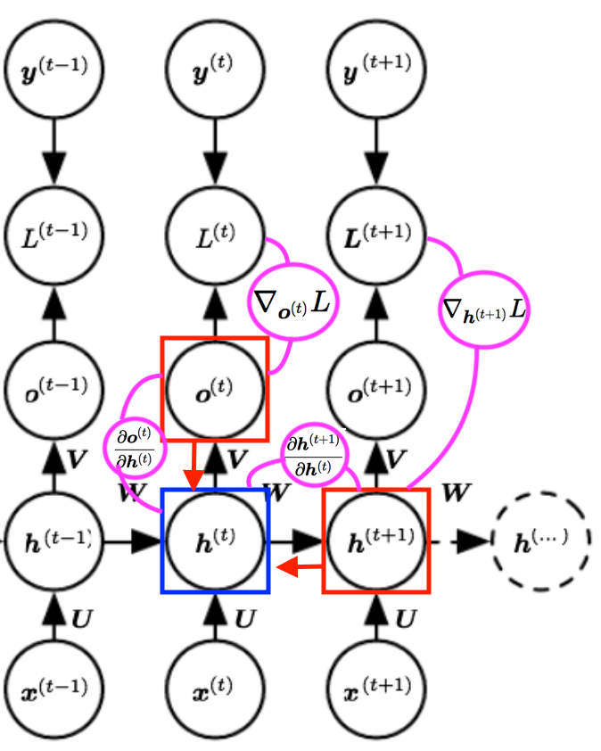
\(\begin{align} L(y, \hat{y}) &= \sum_{t} L^{(t)} = -\sum_{t} \log \hat{y}_ t = -\sum_{t} \log p_{\text {model }}\left(y^{(t)} |\left\{\boldsymbol{x}^{(1)}, \ldots, \boldsymbol{x}^{(t)}\right\}\right) \\ \hat{y}_ t &= \text{softmax}(o_t) \\ dy_{\tau} &= \frac{\partial L}{\partial L^{(t)}}=1 \\ do_t &= g_y'(o_t) = \text{softmax}'(o_t) = \hat{y}_{i}^{(t)}-\mathbf{1}_{i=y^{(t)}} \\ dh_{\tau} &= W_{oh}^T do_t \\ dh_t &= \left(\frac{\partial \boldsymbol{h}^{(t+1)}}{\partial \boldsymbol{h}^{(t)}}\right)^{\top}\left(\nabla_{\boldsymbol{h}^{(t+1)}} L\right)+\left(\frac{\partial \boldsymbol{o}^{(t)}}{\partial \boldsymbol{h}^{(t)}}\right)^{\top}\left(\nabla_{\boldsymbol{o}^{(t)}} L\right) = \boldsymbol{W_{hh}}^{\top} \operatorname{diag}\left(1-\left(\boldsymbol{h}^{(t+1)}\right)^{2}\right)\left(\nabla_{\boldsymbol{h}^{(t+1)}} L\right)+\boldsymbol{W_{oh}}^{\top}\left(\nabla_{\boldsymbol{o}^{(t)}} L\right) \\ du_t &= dh_t · g_h'(u_t) = dh_t · \operatorname{tanh}'(u_t) = dh_t · \sum_{t} \operatorname{diag}\left(1-\left(h^{(t)}\right)^{2}\right) \\ db_o &= do_t \\ dW_{oh} &= do_th_t^T \\ dW_{hx} &= du_tx_t^T \\ db_h &= du_t \\ dW_{hh} &= du_th_{t-1}^T \\ dh_{t-1} &= W_{hh}^T du_t \end{align}\)Notes:
- \(dh_{\tau}\): We need to get the gradient of \(h\) at the last node/time-step \(\tau\) i.e. \(h_{\tau}\)
- \(dh_t\): We can then iterate backward in time to back-propagate gradients through time, from \(t=\tau-1\) down to \(t=1\), noting that \(h^{(t)}(\text { for } t<\tau)\) has as descendants both \(\boldsymbol{o}^{(t)}\) and \(\boldsymbol{h}^{(t+1)}\).
- Backpropagation Through Time:
- We can think of the recurrent net as a layered, feed-forward net with shared weights and then train the feed-forward net with (linear) weight constraints.
- We can also think of this training algorithm in the time domain:
- The forward pass builds up a stack of the activities of all the units at each time step
- The backward pass peels activities off the stack to compute the error derivatives at each time step
- After the backward pass we add together the derivatives at all the different times for each weight.
Complexity:
Linear in the length of the longest sequence.
Minibatching can be inefficient as the sequences in a batch may have different lengths.Can be alleviated w/ padding.
-
Truncated BPTT:
Same as BPTT, but tries to avoid the problem of long sequences as inputs. It does that by “breaking” the gradient flow every nth time-step (if input is article, then n could be average length of a sentence), thus, avoiding problems of (1) Memory (2) Exploding Gradient.Downsides:
If there are dependencies between the segments where BPTT was truncated they will not be learned because the gradient doesn’t flow back to teach the hidden representation about what information was useful.Complexity:
Constant in the truncation length \(T\).
Minibatching is efficient as all sequences have length \(T\).Notes:
- In TBPTT, we Forward Propagate through-the-break/between-segments normally (through the entire comp-graph). Only the back-propagation is truncated.
- Mini-batching on a GPU is an effective way of speeding up big matrix vector products 2. RNNLMs have two such products that dominate their computation: the recurrent matrix \(V\) and the softmax matrix \(W\).
LSTMS:
- The core of the history/memory is captured in the cell-state \(c_{n}\) instead of the hidden state \(h_{n}\).
- (&) Key Idea: The update to the cell-state \(c_{n}=c_{n-1}+\operatorname{tanh}\left(V\left[w_{n-1} ; h_{n-1}\right]+b_{c}\right)\) here are additive. (differentiating a sum gives the identity) Making the gradient flow nicely through the sum. As opposed to the multiplicative updates to \(h_n\) in vanilla RNNs.
There is non-linear funcs applied to the history/context cell-state. It is composed of linear functions. Thus, avoids gradient shrinking.
- In the recurrency of the LSTM the activation function is the identity function with a derivative of 1.0. So, the backpropagated gradient neither vanishes or explodes when passing through, but remains constant.
- By the selective read, write and forget mechanism (using the gating architecture) of LSTM, there exist at least one path, through which gradient can flow effectively from \(L\) to \(\theta\). Hence no vanishing gradient.
- However, one must remember that, this is not the case for exploding gradient. It can be proved that, there can exist at-least one path, thorough which gradient can explode.
- LSTM decouples cell state (typically denoted by c) and hidden layer/output (typically denoted by h), and only do additive updates to c, which makes memories in c more stable. Thus the gradient flows through c is kept and hard to vanish (therefore the overall gradient is hard to vanish). However, other paths may cause gradient explosion.
- The Vanishing gradient solution for LSTM is known as Constant Error Carousel.
- Why can RNNs with LSTM units also suffer from “exploding gradients”?
- LSTMs (Lec Oxford)
Important Links:
The unreasonable effectiveness of Character-level Language Models
character-level language model with a Vanilla Recurrent Neural Network, in Python/numpy
Visualizing and Understanding Recurrent Networks - Karpathy Lec
Cool LSTM Diagrams - blog
Illustrated Guide to Recurrent Neural Networks: Understanding the Intuition
Code LSTM in Python
Mikolov Thesis: STATISTICAL LANGUAGE MODELS BASED ON NEURAL NETWORKS
RNNs Extra!
-
- Vanishing/Exploding Gradients:
-
- Exploding Gradients:
- Truncated BPTT
- Clip gradients at threshold
- RMSprop to adjust learning rate
- Vanishing Gradient:
- Harder to detect
- Weight initialization
- ReLu activation functions
- RMSprop
- LSTM, GRUs
- Exploding Gradients:
-
- Applications:
-
- NER
- Entity Level Sentiment in context
- Opinionated Expressions
-
- Bidirectional RNNs:
-
- Motivation:
For classification we need to incorporate information from words both preceding and following the word being processed
- Motivation:
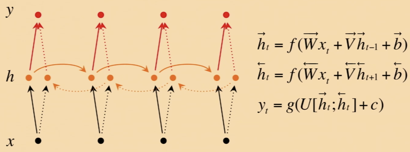
- \(\:\:\:\:\) Here \(h = [\overrightarrow{h};\overleftarrow{h}]\) represents (summarizes) the past and the future around a single token.
-
- Deep Bidirectional RNNs:
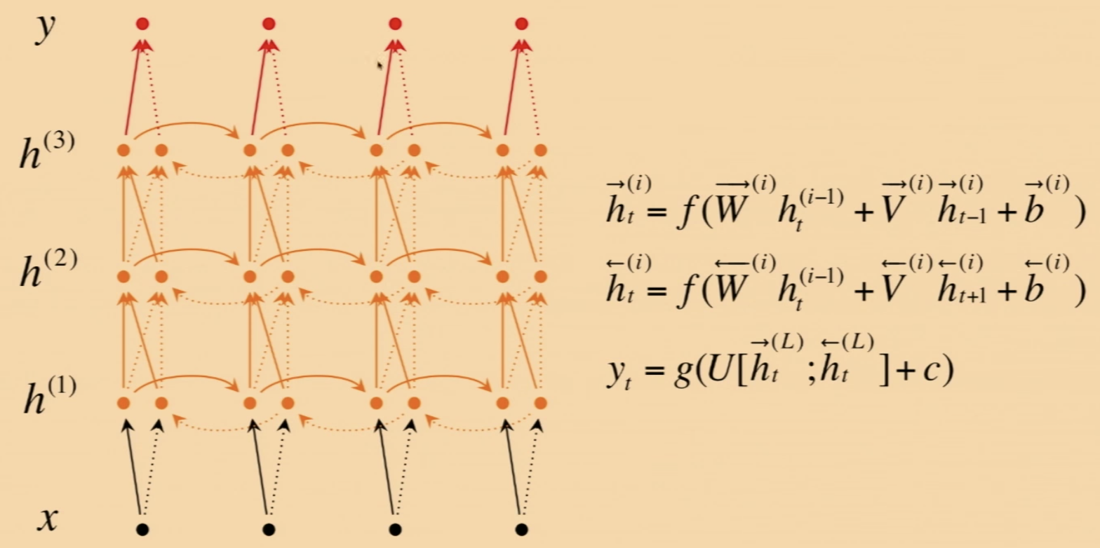
- \(\:\:\:\:\:\) Each memory layer passes an intermediate sequential representation to the next.
-
- Math to Code:
- The Parameters: \(\{W_{hx}, W_{hh}, W_{oh} ; b_h, b_o, h_o\}\)
- \[\begin{align} h_t &= \phi(W_{hx}x_t + W_{hh}h_{t-1} + b_h) \\ h_t &= \phi(\begin{bmatrix} W_{hx} & ; & W_{hh} \end{bmatrix} \begin{bmatrix} x_t \\ ; \\ h_{t-1} \end{bmatrix} + b_h) \end{align}\]
- \[y_t = \phi'(W_{oh}h_t + b_o)\]
-
- Initial States:
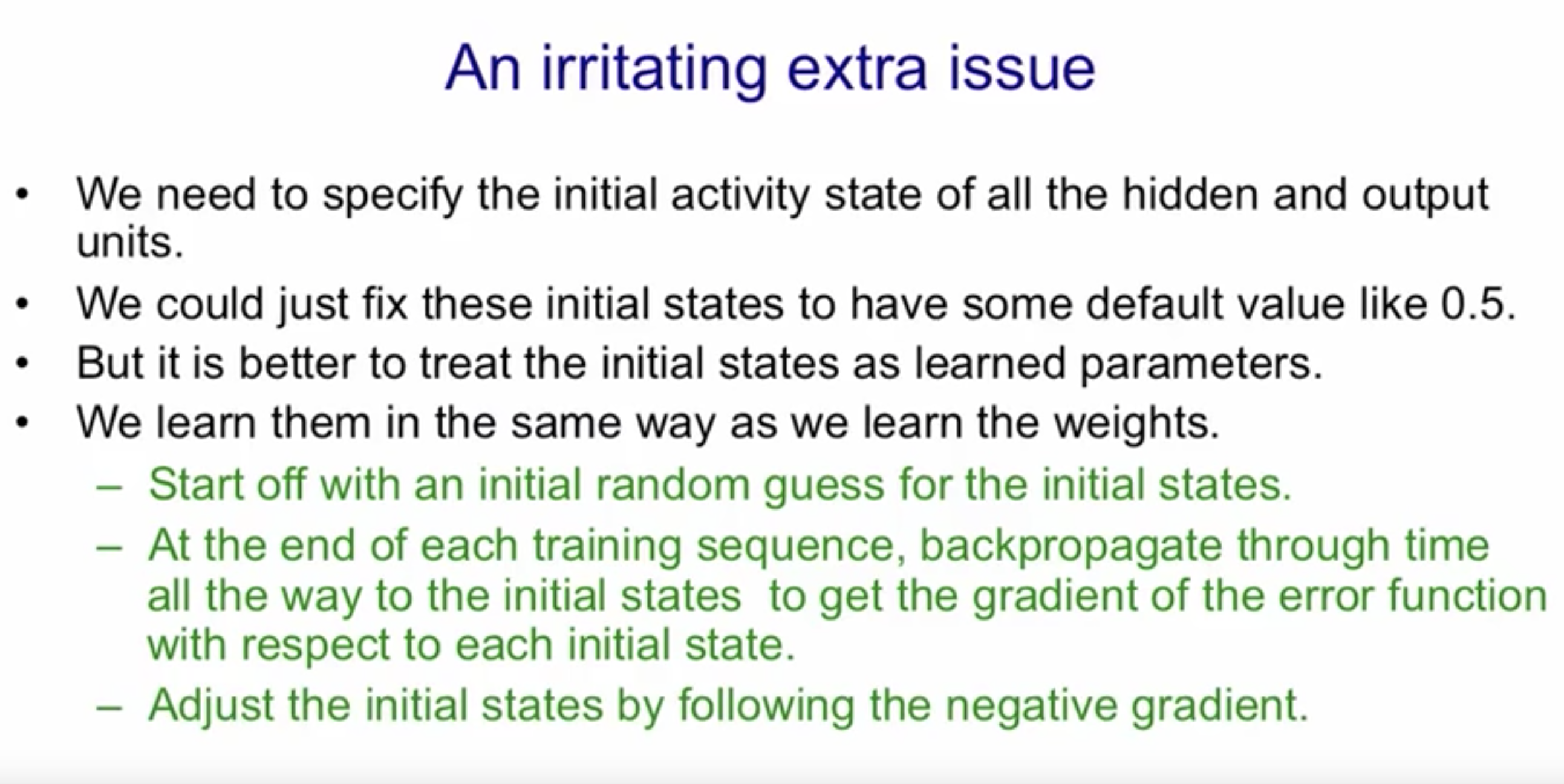
-
- Specifying the Initial States:
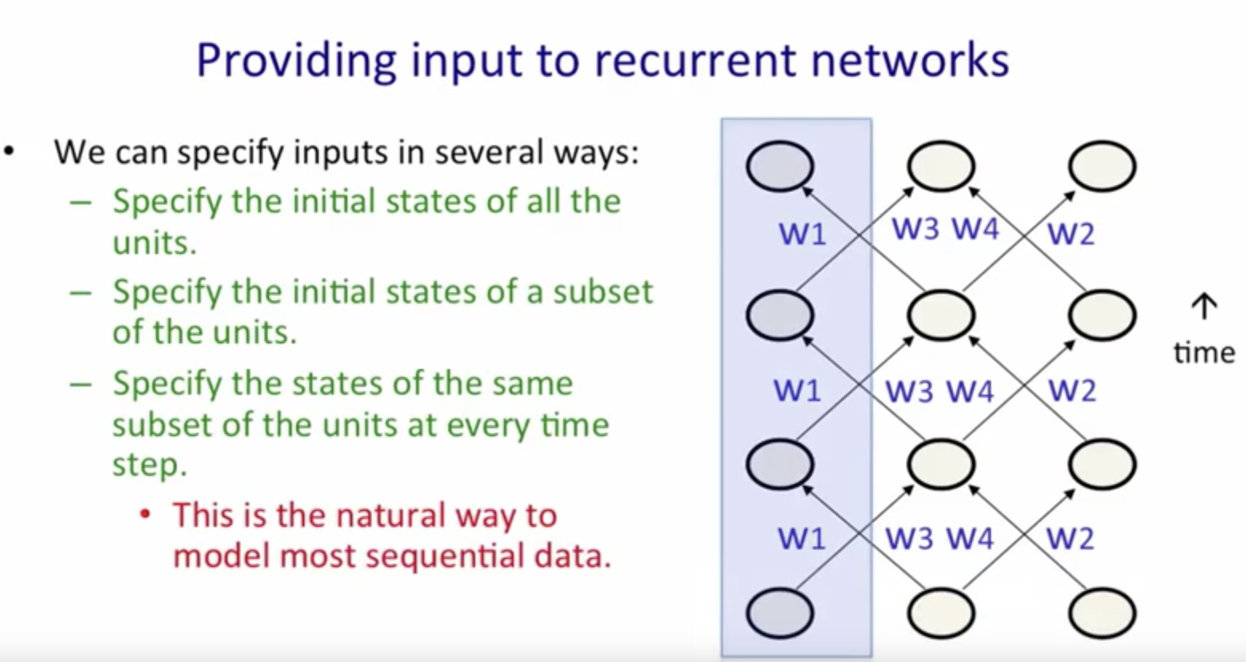
-
- Teaching Signals:
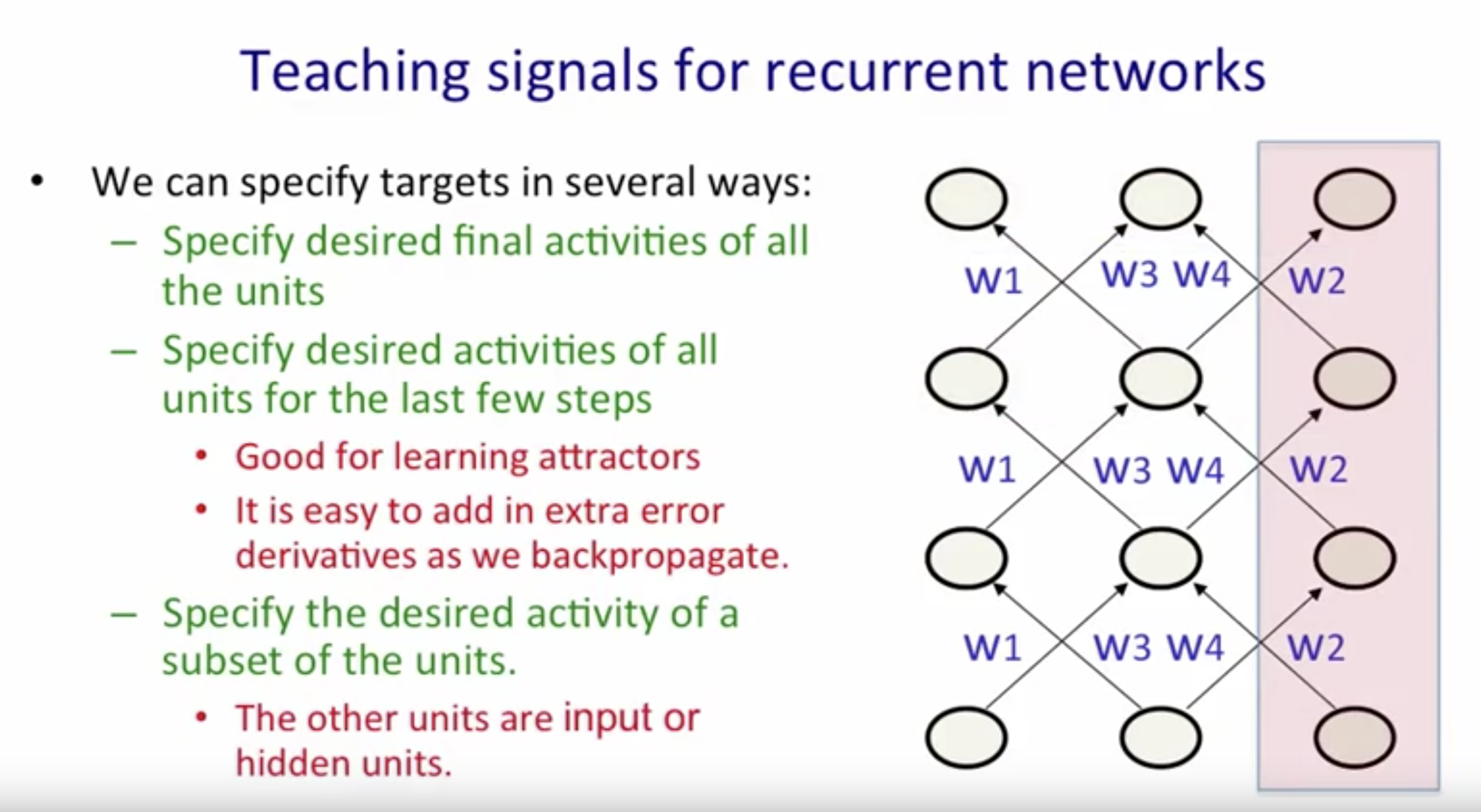
-
- Vanishing/Exploding Gradients:
-
- Exploding Gradients:
- Truncated BPTT
- Clip gradients at threshold
- RMSprop to adjust learning rate
- Vanishing Gradient:
- Harder to detect
- Weight initialization
- ReLu activation functions
- RMSprop
- LSTM, GRUs
- Exploding Gradients:
-
- Rectifying the Vanishing/Exploding Gradient Problem:
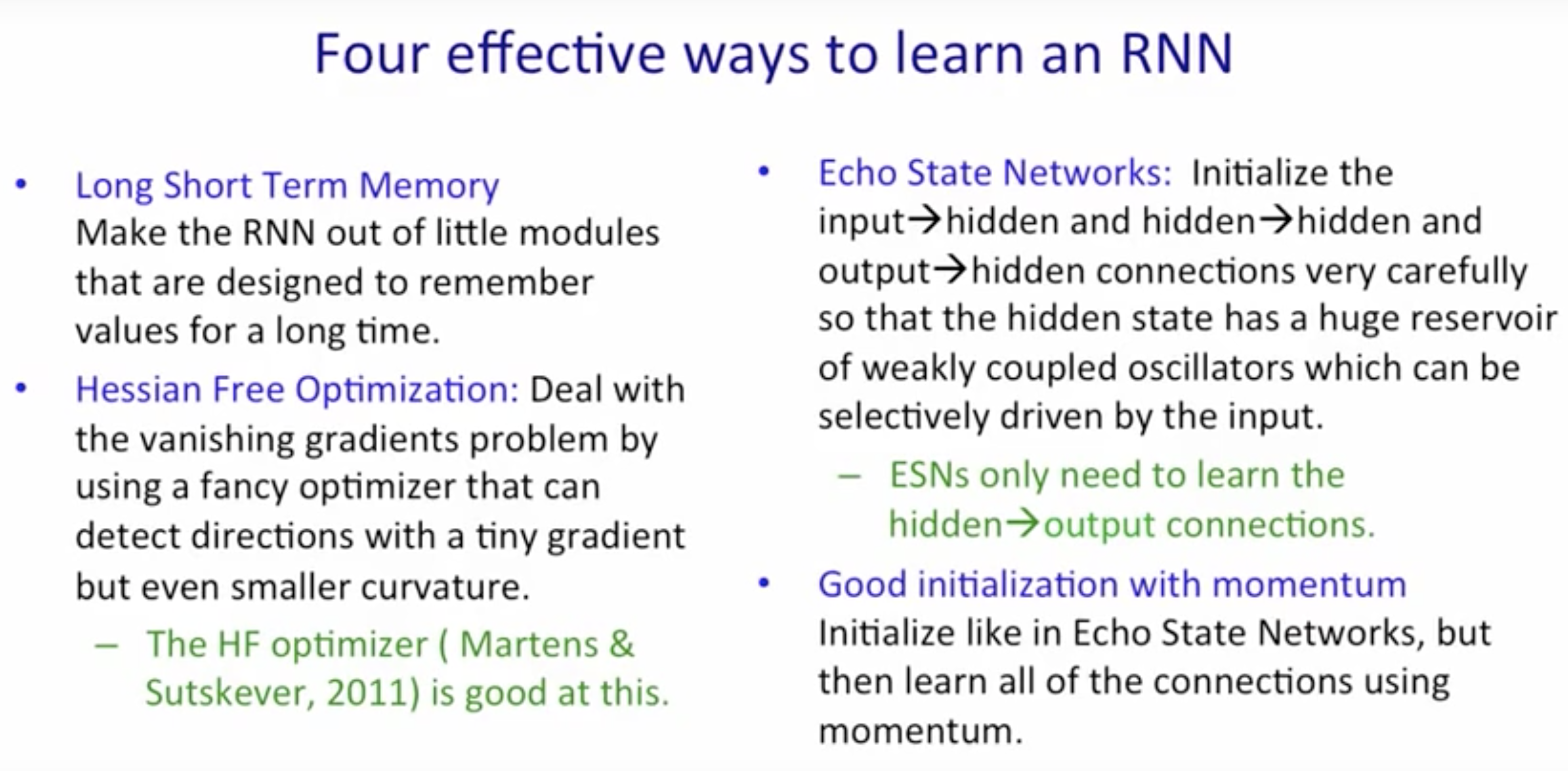
-
- Linearity of BackProp:
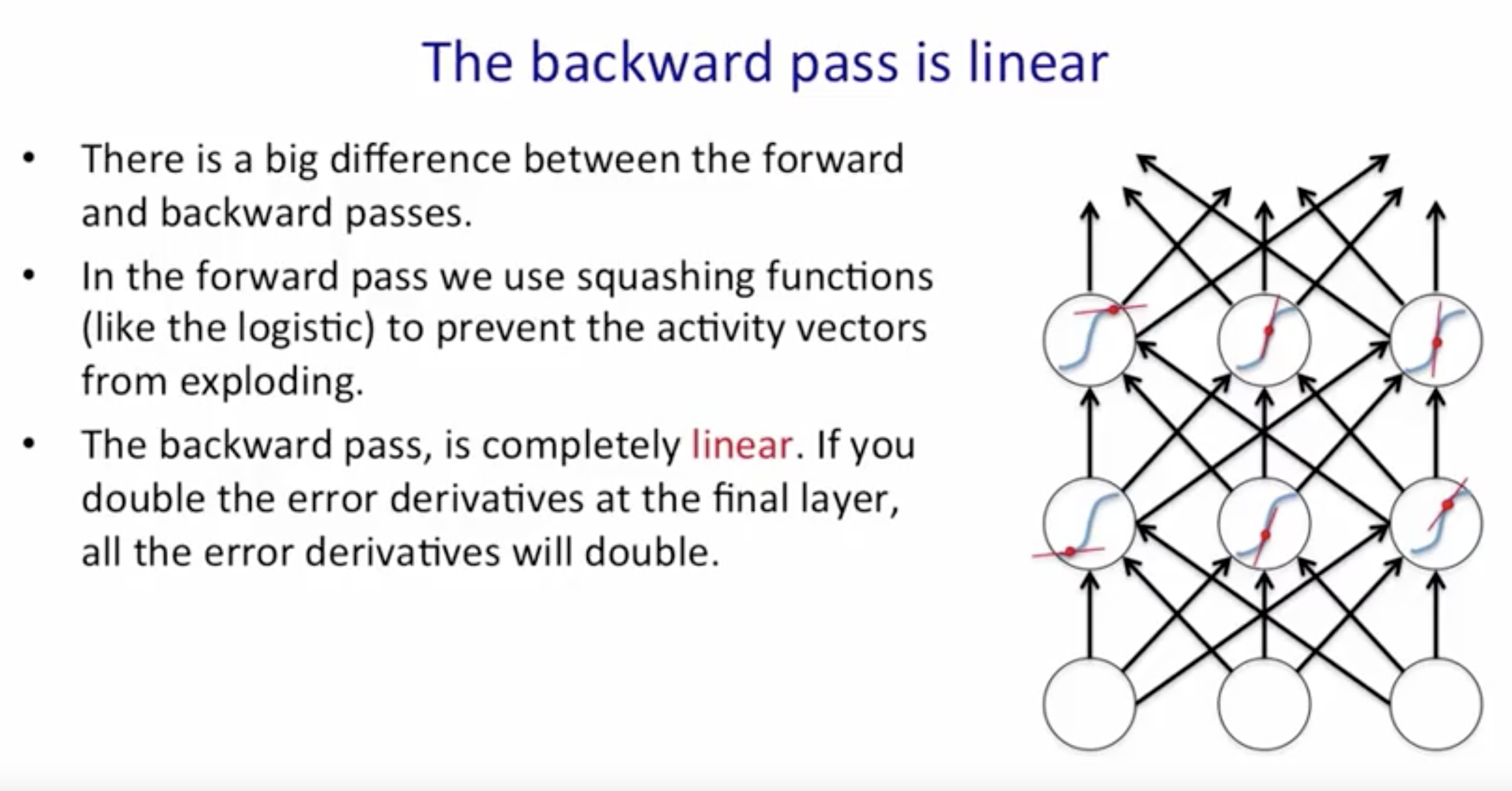
- The derivative update are also Correlated which is bad for SGD.
-
the problem of assigning a probability to a string and text compression is exactly the same problem so if you have a good language model you also have a good text compression algorithm and both we think of it in terms of the number of bits we can compress our sequence into. ↩
-
By making them Matrix-Matrix products instead. ↩
