Ahmad Badary

Introduction to Speech Recognition

The Methods and Models of Speech Recognition

Transitioning into Deep Learning

Connectionist Temporal Classification

LAS - Seq2Seq with Attention

Online Seq2Seq Models

Real-World Applications

Building ASR Systems

Introduction to Speech

Probabilistic Speech Recognition:

Statistical ASR has been introduced/framed by Frederick Jelinek in his famous paper Continuous Speech Recognition by Statistical Methods who framed the problem as an information theory problem.

We can view the problem of ASR as a sequence labeling problem, and, so, use statistical models (such as HMMs) to model the conditional probabilities between the states/words by viewing speech signal as a piecewise stationary signal or a short-time stationary signal.
- Representation: we represent the speech signal as an observation sequence $o = \{o_t\}$
- Goal: find the most likely word sequence $\hat{w}$
- Set-Up:
  - The system has a set of discrete states
  - The transitions from state to state are markovian and are according to the transition probabilities
    
    Markovian: Memoryless
  - The Acoustic Observations when making a transition are conditioned on the state alone $P(o_t \vert c_t)$
  - The goal is to recover the state sequence and, consequently, the word sequence
Speech Problems and Considerations:
- ASR:
  - Spontaneous vs Read speech
  - Large vs Small Vocabulary
  - Continuous vs Isolated Speech
    
    Continuous Speech is harder due to Co-Articulation
  - Noisy vs Clear input
  - Low vs High Resources
  - Near-field vs Far-field input
  - Accent-independence
  - Speaker-Adaptive vs Stand-Alone (speaker-independent)
  - The cocktail party problem
- TTS:
  - Low Resource
  - Realistic prosody
- Speaker Identification
- Speech Enhancement
- Speech Separation
Acoustic Representation:
What is speech?
- Waves of changing air pressure - Longitudinal Waves (consisting of compressions and rarefactions)
- Realized through excitation from the vocal cords
- Modulated by the vocal tract and the articulators (tongue, teeth, lips)
- Vowels are produced with an open vocal tract (stationary)
  
  parametrized by position of tongue
- Consonants are constrictions of vocal tract
- They get converted to Voltage with a microphone
- They are sampled (and quantized) with an Analogue to Digital Converter
Speech as waves:
- Human hearing range is: $~50 HZ-20 kHZ$
- Human speech range is: $~85 HZ-8 kHZ$
- Telephone speech sampling is $8 kHz$ and a bandwidth range of $300 Hz-4 kHz$
- 1 bit per sample is intelligible
- Contemporary Speech Processing mostly around 16 khz 16 bits/sample
  
  A lot of data to handle
Speech as digits (vectors):
- We seek a low-dimensional representation to ease the computation
- The low-dimensional representation needs to be invariant to:
  - Speaker
  - Background noise
  - Rate of Speaking
  - etc.
- We apply Fourier Analysis to see the energy in different frequency bands, which allows analysis and processing
  - Specifically, we apply windowed short-term Fast Fourier Transform (FFT)
    
    e.g. FFT on overlapping $25ms$ windows (400 samples) taken every $10ms$
    
    Each frame is around 25ms of speech
- FFT is still too high-dimensional
  - We Downsample by local weighted averages on mel scale non-linear spacing, an d take a log:
    $m = 1127 \ln(1+\dfrac{f}{700})$
  - This results in log-mel features, $40+$ dimensional features per frame
    
    Default for NN speech modelling
Speech dimensionality for different models:
- Gaussian Mixture Models (GMMs): 13 MFCCs
  - MFCCs - Mel Frequency Cepstral Coefficients: are the discrete cosine transformation (DCT) of the mel filterbank energies | Whitened and low-dimensional.
    They are similar to Principle Components of log spectra.
    GMMs used local differences (deltas) and second-order differences (delta-deltas) to capture the dynamics of the speech $(13 \times 3 \text{ dim})$
- FC-DNN: 26 stacked frames of PLP
  - PLP - Perceptual Linear Prediction: a common alternative representation using Linear Discriminant Analysis (LDA)
    
    Class aware PCA
- LSTM/RNN/CNN: 8 stacked frames of PLP
Speech as Communication:
- Speech Consists of sentences (in ASR we usually talk about “utterances”)
- Sentences are composed of words
- Minimal unit is a “phoneme” Minimal unit that distinguishes one word from another.
  - Set of 40-60 distinct sounds.
  - Vary per language
  - Universal representations:
    
    IPA : international phonetic alphabet
    
    X-SAMPA : (ASCII)
- Homophones : distinct words with the same pronunciation. (e.g. “there” vs “their”)
- Prosody : How something is said can convey meaning. (e.g. “Yeah!” vs “Yeah?”)
Microphones and Speakers:
- Microphones:
  - Their is a Diaphragm in the Mic
  - The Diaphragm vibrates with air pressure
  - The diaphragm is connected to a magnet in a coil
  - The magnet vibrates with the diaphragm
  - The coil has an electric current induced by the magnet based on the vibrations of the magnet
- Speakers:
  - The electric current flows from the sound-player through a wire into a coil
  - The coil has a metal inside it
  - The metal becomes magnetic and vibrates inside the coil based on the intensity of the current
  - The magnetized metal is attached to a cone that produces the sound
(Approximate) History of ASR:
- 1960s Dynamic Time Warping
- 1970s Hidden Markov Models
- Multi-layer perceptron 1986
- Speech recognition with neural networks 1987-1995
- Superseded by GMMs 1995-2009
- Neural network features 2002—
- Deep networks 2006— (Hinton, 2002)
- Deep networks for speech recognition:
  - Good results on TIMIT (Mohamed et al., 2009)
  - Results on large vocabulary systems 2010 (Dahl et al., 2011) * Google launches DNN ASR product 2011
  - Dominant paradigm for ASR 2012 (Hinton et al., 2012)
- Recurrent networks for speech recognition 1990, 2012 - New models (CTC attention, LAS, neural transducer)
Datasets:
- TIMIT:
  - Hand-marked phone boundaries are given
  - 630 speakers $\times$ 10 utterances
- Wall Street Journal (WSJ) 1986 Read speech. WSJO 1991, 30k vocab
- Broadcast News (BN) 1996 104 hours
- Switchboard (SWB) 1992. 2000 hours spontaneous telephone speech - 500 speakers
- Google voice search - anonymized live traffic 3M utterances 2000 hours hand-transcribed 4M vocabulary. Constantly refreshed, synthetic reverberation + additive noise
- DeepSpeech 5000h read (Lombard) speech + SWB with additive noise.
- YouTube 125,000 hours aligned captions (Soltau et al., 2016)
Development:

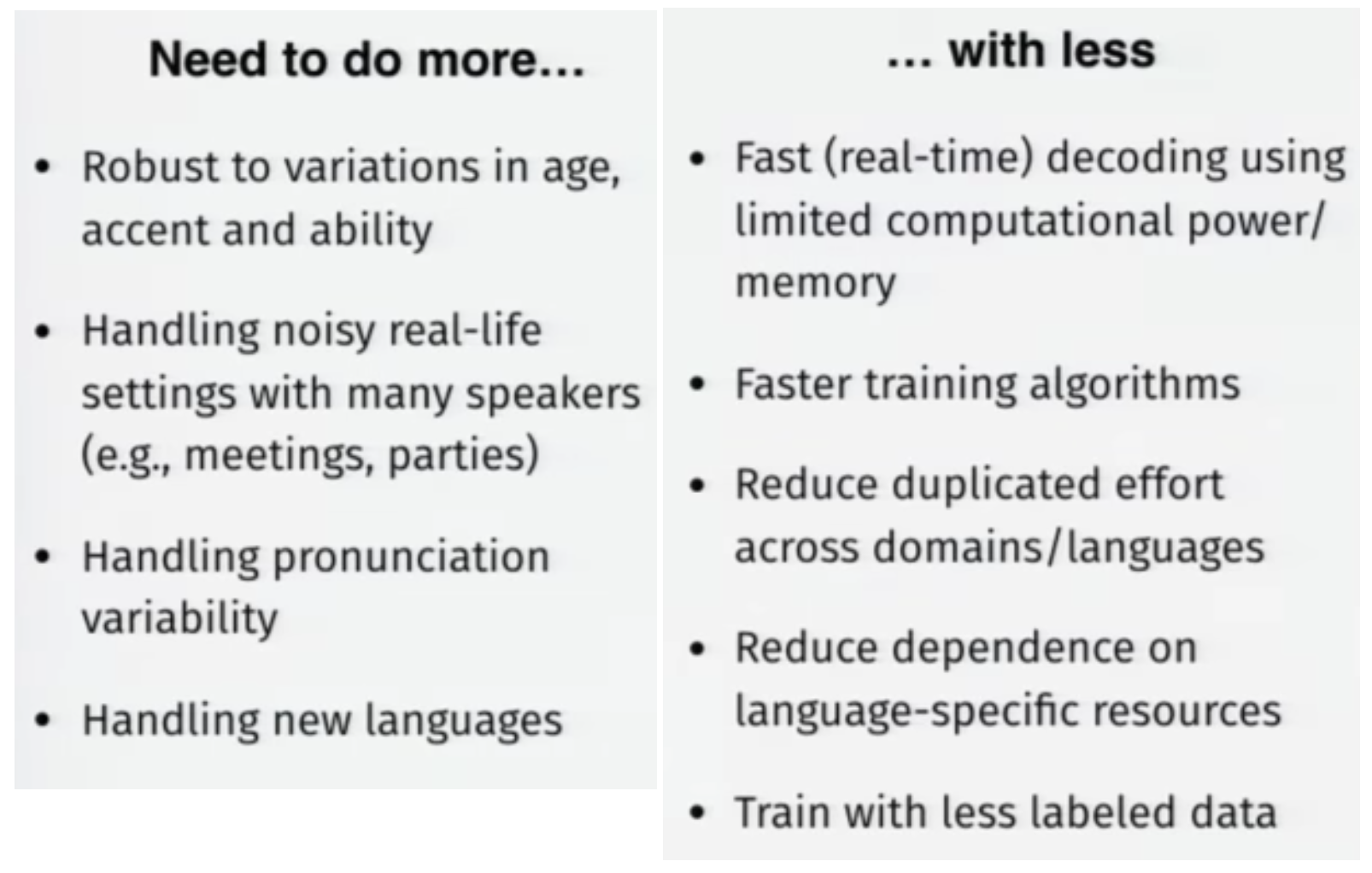
The Methods and Models of Speech Recognition

Probabilistic Speech Recognition:

Statistical ASR has been introduced/framed by Frederick Jelinek in his famous paper Continuous Speech Recognition by Statistical Methods who framed the problem as an information theory problem.

We can view the problem of ASR as a sequence labeling problem, and, so, use statistical models (such as HMMs) to model the conditional probabilities between the states/words by viewing speech signal as a piecewise stationary signal or a short-time stationary signal.
- Representation: we represent the speech signal as an observation sequence $o = \{o_t\}$
- Goal: find the most likely word sequence $\hat{w}$
- Set-Up:
  - The system has a set of discrete states
  - The transitions from state to state are markovian and are according to the transition probabilities
    
    Markovian: Memoryless
  - The Acoustic Observations when making a transition are conditioned on the state alone $P(o_t \vert c_t)$
  - The goal is to recover the state sequence and, consequently, the word sequence
Fundamental Equation of Speech Recognition:

We set the decoders output as the most likely sequence $\hat{w}$ from all the possible sequences, $\mathcal{S}$, for an observation sequence $o$:

\[\begin{align} \hat{w} & = \mathrm{arg } \max_{w \in \mathcal{S}} P(w \vert o) & (1) \\ & = \mathrm{arg } \max_{w \in \mathcal{S}} P(o \vert w) P(w) & (2) \end{align}\]

The Conditional Probability of a sequence of observations given a sequence of (predicted) word is a product (or sum of logs) of an Acoustic Model ($p(o \vert w)$) and a Language Model ($p(w)$) scores.

The Acoustic Model can be written as the following product:

\[P(o \vert w) = \sum_{d,c,p} P(o \vert c) P(c \vert p) P(p \vert w)\]

where $p$ is the phone sequence and $c$ is the state sequence.
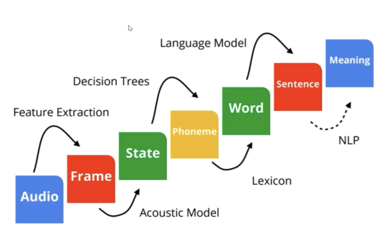
Speech Recognition as Transduction:

The problem of speech recognition can be seen as a transduction problem - mapping different forms of energy to other forms (representations).
Basically, we are going from Signal to Language.
Gaussian Mixture Models:
- Dominant paradigm for ASR from 1990 to 2010
- Model the probability distribution of the acoustic features for each state.
  $P(o_t \vert c_i) = \sum_j w_{ij} N(o_t; \mu_{ij}, \sigma_{ij})$
- Often use diagonal covariance Gaussians to keep number of parameters under control.
- Train by the E-M (Expectation Maximization) algorithm (Dempster et al., 1977) alternating:
  - M: forced alignment computing the maximum-likelihood state sequence for each utterance
  - E: parameter $(\mu , \sigma)$ estimation
- Complex training procedures to incrementally fit increasing numbers of components per mixture:
  - More components, better fit - 79 parameters component.
- Given an alignment mapping audio frames to states, this is parallelizable by state.
- Hard to share parameters/data across states.
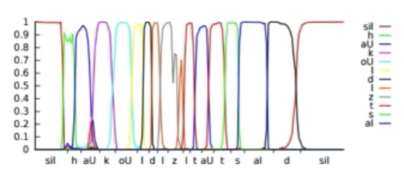
Forced Alignment:
- Forced alignment uses a model to compute the maximum likelihood alignment between speech features and phonetic states.
- For each training utterance, construct the set of phonetic states for the ground truth transcription.
- Use Viterbi algorithm to find ML monotonic state sequence
- Under constraints such as at least one frame per state.
- Results in a phonetic label for each frame.
- Can give hard or soft segmentation.
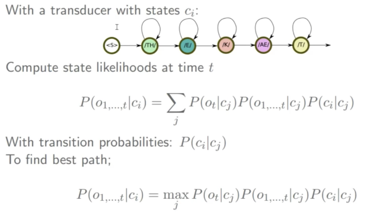
- Decoding:
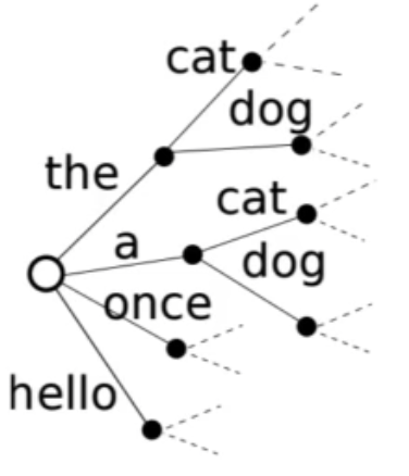
  - Speech recognition Unfolds in much the same way.
  - Now we have a graph instead of a straight-through path.
  - Optional silences between words Alternative pronunciation paths.
  - Typically use max probability, and work in the log domain.
  - Hypothesis space is huge, so we only keep a “beam” of the best paths, and can lose what would end up being the true best path.
Neural Networks in ASR:
- Two Paradigms of Neural Networks for Speech:
  - Use neural networks to compute nonlinear feature representations:
    
    “Bottleneck” or “tandem” features (Hermansky et al., 2000)
    
    Low-dimensional representation is modelled conventionally with GMMs.
    
    Allows all the GMM machinery and tricks to be exploited.
    
    Bottleneck features outperform Posterior features (Grezl et al. 2017)
    
    Generally, DNN features + GMMs reach the same performance as hybrid DNN-HMM systems but are much more complex
  - Use neural networks to estimate phonetic unit probabilities
Hybrid Networks:
- Train the network as a classifier with a softmax across the phonetic units
- Train with cross-entropy
- Softmax:
\[y(i) = \dfrac{e^{\psi(i, \theta)}}{\sum_{j=1}^N e^{\psi(j, \theta)}}\]
- We converge to/learn the posterior probability across phonetic states:
\[P(c_i \vert o_t)\]
- We, then, model $P(o \vert c)$ with a Neural-Net instead of a GMM:
  
  We can ignore $P(o_t)$ since it is the same for all decoding paths
\[\begin{align} P(o \vert c) & = \prod_t P(o_t \vert c_t) & (3) \\ P(o_t \vert c_t) & = \dfrac{P(c_t \vert o_t) P(o_t)}{P(c_t)} & (4) \\ & \propto \dfrac{P(c_t \vert o_t)}{P(c_t)} & (5) \\ \end{align}\]
- The log scaled posterior from the last term:
\[\log P(o_t \vert c_t) = \log P(c_t \vert o_t) - \alpha \log P(c_t)\]
- Empirically, a prior smoothing on $\alpha$ $(\alpha \approx 0.8)$ works better
- Input Features:
  - NN can handle high-dimensional, correlated, features
  - Use (26) stacked filterbank inputs (40-dim mel-spaced filterbanks)
- NN Architectures for ASR:
  - Fully-Connected DNN
  - CNNs:
    
    Time delay neural networks:
    
    Waibel et al. (1989)
    
    Dilated convolutions (Peddinti et al., 2015)
    
    Pooling in time results in a loss of information.
    Pooling in frequency domain is more tolerable
    
    CNNs in time or frequency domain:
    
    Abdel-Hamid et al. (2014)
    
    Sainath et al. (2013)
    
    Wavenet (van den Oord et al., 2016)
  - RNNs :
    
    RNN (Robinson and Fallside, 1991)
    
    LSTM Graves et al. (2013)
    
    Deep LSTM-P Sak et al. (2014b)
    
    CLDNN (Sainath et al , 2015a)
    
    GRU. DeepSpeech 1/2 (Amodei et al., 2015)
    
    Tips :
    
    Bidirectional (Schuster and Paliwal, 1997) helps, but introduces latency.
    
    Dependencies not long at speech frame rates (100Hz).
    
    Frame stacking and down-sampling help.
Sequence Discriminative Training:
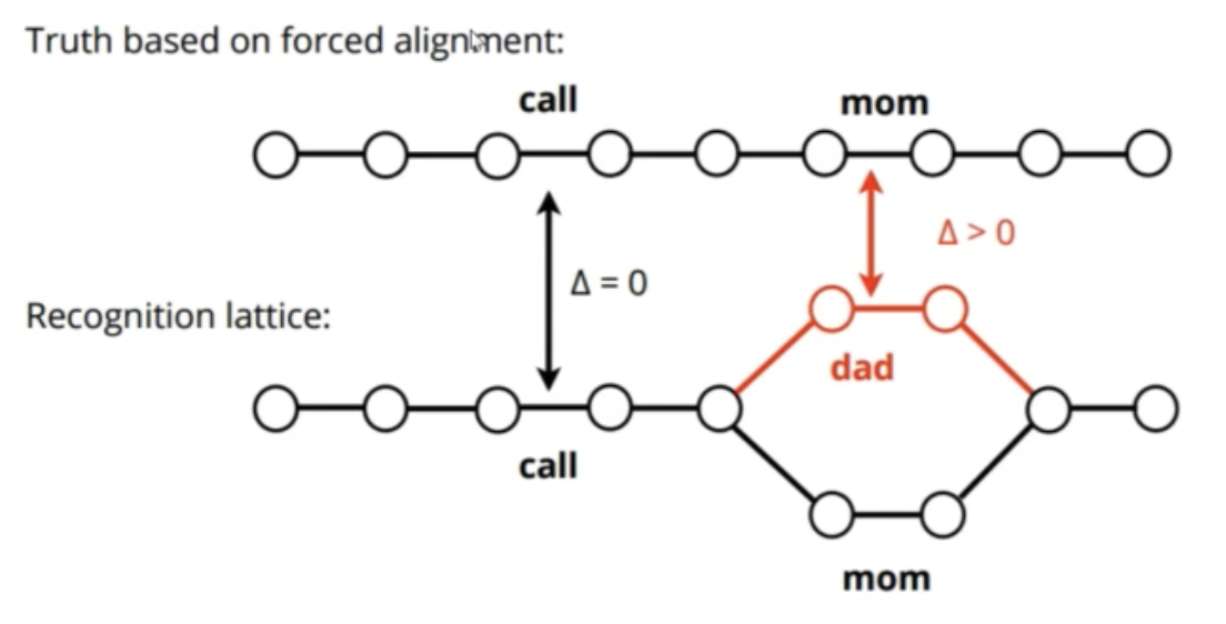
- Conventional training uses Cross-Entropy loss — Tries to maximize probability of the true state sequence given the data.
- We care about Word Error Rate of the complete system.
- Design a loss that’s differentiable and closer to what we care about.
- Applied to neural networks (Kingsbury, 2009)
- Posterior scaling gets learnt by the network.
- Improves conventional training and CTC by $\approx 15%$ relative.
- bMMI, sMBR(Povey et al., 2008)
Asynchronous:

Transitioning into Deep Learning

Classical Approach:

Classically, Speech Recognition was developed as a big machine incorporating different models from different fields.
The models were statistical and they started from text sequences to audio features.
Typically, a generative language model is trained on the sentences for the intended language, then, to make the features, pronunciation models, acoustic models, and speech processing models had to be developed. Those required a lot of feature engineering and a lot of human intervention and expertise and were very fragile.

Recognition was done through Inference: Given audio features $\mathbf{X}=x_1x_2...x_t$ infer the most likely tedxt sequence $\mathbf{Y}^\ast=y_1y_2...y_k$ that caused the audio features.

\[\displaystyle{\mathbf{Y}^\ast =\mathrm{arg\,min}_{\mathbf{Y}} p(\mathbf{X} \vert \mathbf{Y}) p(\mathbf{Y})}\]
The Neural Network Age:

Researchers realized that each of the (independent) components/models that make up the ASR can be improved if it were replaced by a Neural Network Based Model.
The Problem with the component-based System:
- Each component/model is trained independently, with a different objective
- Errors in one component may not behave well with errors in another component
Solution to the Component-Based System:
We aim to train models that encompass all of these components together, i.e. End-to-End Model:
- Connectionist Temporal Classification (CTC)
- Sequence-to-Sequence Listen Attend and Spell (LAS)
End-to-End Speech Recognition:

We treat End-to-End Speech Recognition as a modeling task.

Given Audio $\mathbf{X}=x_1x_2...x_t$ (audio/processed spectogram) and corresponding output text $\mathbf{Y}=y_1y_2...y_k$ (transcript), we want to learn a Probabilistic Model $p(\mathbf{Y} \vert \mathbf{X})$
Deep Learning - What’s new?
- Algorithms:
  - Direct modeling of context-dependent (tied triphone states) through the DNN
  - Unsupervised Pre-training
  - Deeper Networks
  - Better Architectures
    
    Data:
  - Larger Data
    
    Computation:
    
    GPUs
    
    TPUs
    
    Training Criterion:
  - Cross-Entropy -> MMI Sequence -level
    
    Features:
  - Mel-Frequency Cepstral Coefficients (MFCC) -> FilterBanks
    
    Training and Regularization:
  - Batch Norm
  - Distributed SGD
  - Dropout
    
    Acoustic Modelling:
  - CNN
  - CTC
  - CLDNN
    
    Language Modelling:
  - RNNs
  - LSTM
    
    DATA:
  - More diverse - Noisy, Accents, etc.

Connectionist Temporal Classification

Motivation:
- RNNs require a target output at each time step
- Thus, to train an RNN, we need to segment the training output (i.e. tell the network which label should be output at which time-step)
- This problem usually arises when the timing of the input is variable/inconsistent (e.g. people speaking at different rates/speeds)
Connectionist Temporal Classification (CTC):

CTC is a type of neural network output and associated scoring function, for training recurrent neural networks (RNNs) such as LSTM networks to tackle sequence problems where the timing is variable.

Due to time variability, we don’t know the alignment of the input with the output.
Thus, CTC considers all possible alignments.
Then, it gets a closed formula for the probability of all these possible alignments and maximizes it.
Structure:
- Input:
  A sequence of observations
- Output:
  A sequence of labels
Algorithm:
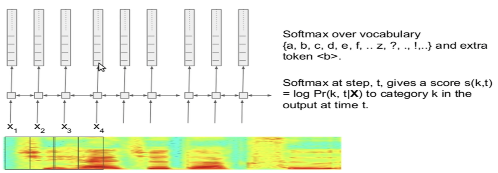
1. Extract the (LOG MEL) Spectrogram from the input
  
  Use raw audio iff there are multiple microphones
2. Feed the Spectogram into a (bi-directional) RNN
3. At each frame, we apply a softmax over the entire vocabulary that we are interested in (plus a blank token), producing a prediction log probability (called the score) for a different token class at that time step.
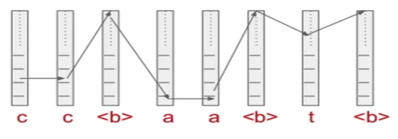
  - Repeated Tokens are duplicated
  - Any original transcript is mapped to by all the possible paths in the duplicated space
  - The Score (log probability) of any path is the sum of the scores of individual categories at the different time steps
  - The probability of any transcript is the sum of probabilities of all paths that correspond to that transcript
  - Dynamic Programming allopws is to compute the log probability $p(\mathbf{Y} \vert \mathbf{X})$ and its gradient exactly.
The Math:

Given a length $T$ input sequence $x$, the output vectors $y_t$ are normalized with the Softmax function, then interpreted as the probability of emitting the label (or blank) with index $k$ at time $t$:

\[P(k, t \vert x) = \dfrac{e^{(y_t^k)}}{\sum_{k'} e^{(y_t^{k'})}}\]

where $y_t^k$ is element $k$ of $y_t$.

A CTC alignment $a$ is a length $T$ sequence of blank and label indices.
The probability $P(a \vert x)$ of $a$ is the product of the emission probabilities at every time-step:

\[P(a \vert x) = \prod_{t=1}^T P(a_t, t \vert x)\]

Denoting by $\mathcal{B}$ an operator that removes first the repeated labels, then the blanks from alignments, and observing that the total probability of an output transcription $y$ is equal to the sum of the probabilities of the alignments corresponding to it, we can write:

\[P(y \vert x) = \sum_{a \in \mathcal{B}^{-1}(y)} P(a \vert x)\:\:\:\:\:\:\:\:\:\:\:\:\:\:\:\:(*)\]

Given a target transcription $y^\ast$, the network can then be trained to minimise the CTC objective function:

\[\text{CTC}(x) = - \log P(y^\ast \vert x)\]
Intuition:

The above ‘integrating out’ over possible alignments eq. $(*)$ is what allows the network to be trained with unsegmented data.
The intuition is that, because we don’t know where the labels within a particular transcription will occur, we sum over all the places where they could occur can be efficiently evaluated and differentiated using a dynamic programming algorithm.
Analysis:

The ASR model consists of an RNN plus a CTC layer.
Jointly, the model learns the pronunciation and acoustic model together.
However, a language model is not learned, because the RNN-CTC model makes strong conditional independence assumptions (similar to HMMs).
Thus, the RNN-CTC model is capable of mapping speech acoustics to English characters but it makes many spelling and grammatical mistakes.
Thus, the bottleneck in the model is the assumption that the network outputs at different times are conditionally independent, given the internal state of the network.
Improvements:
- Add a language model to CTC during training time for rescoring. This allows the model to correct spelling and grammar.
- Use word targets of a certain vocabulary instead of characters
Applications:
- on-line Handwriting Recognition
- Recognizing phonemes in speech audio
- ASR
Tips:
- Continuous realignment - no need for a bootstrap model
- Always use soft targets
- Don’t scale by the posterior
- Produces similar results to conventional training
- Simple to implement in the FST framework
- CTC could learn to delay output on its own in order to improve accuracy:
  - In-practice, tends to align transcription closely
  - This is especially problematic for English letters (spelling)
  - Sol:
    bake limited context into model structure; s.t. the model at time-step $T$ can see only some future frames.
    
    Caveat: may need to compute upper layers quickly after sufficient context arrives.
    Can be easier if context is near top.

LAS - Seq2Seq with Attention

Motivation:

The CTC model can only make predictions based on the data; once it has made a prediction for a given frame, it cannot re-adjust the prediction.

Moreover, the strong independence assumptions that the CTC model makes doesn’t allow it to learn a language model.
Listen, Attend and Spell (LAS):

LAS is a neural network that learns to transcribe speech utterances to characters.
In particular, it learns all the components of a speech recognizer jointly.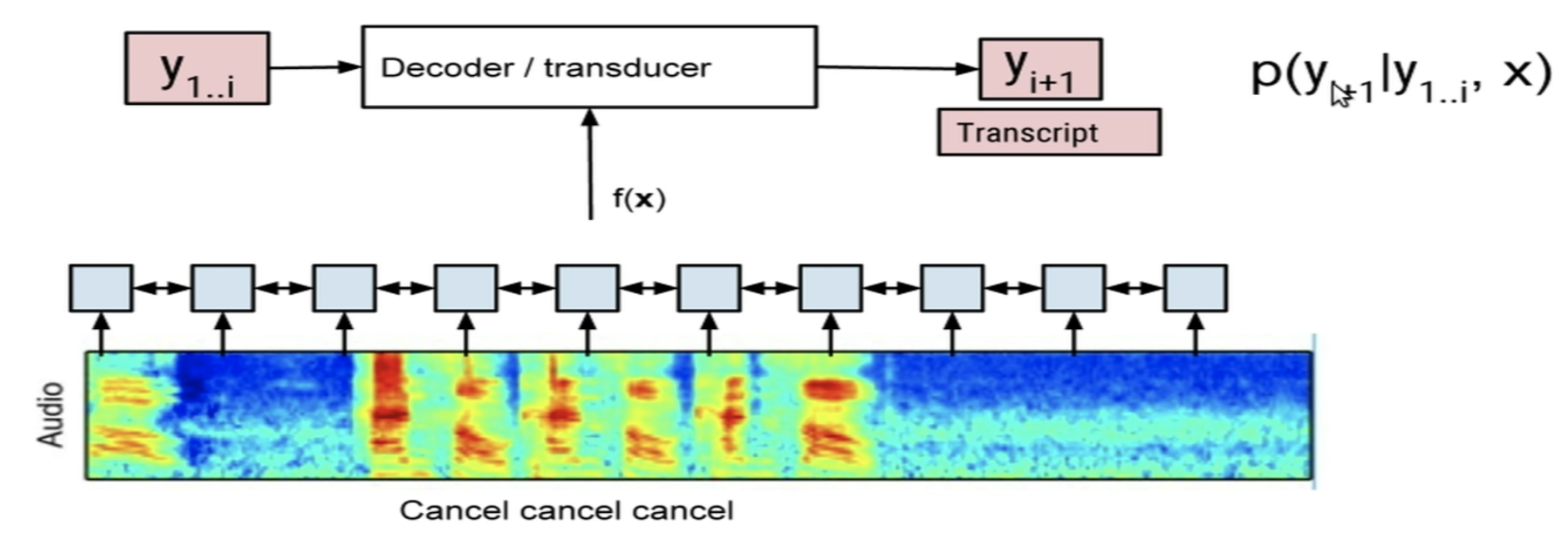

The model is a seq2seq model; it learns a conditional probability of the next label/character given the input and previous predictions $p(y_{i+1} \vert y_{1..i}, x)$.

The approach that LAS takes is similar to that of NMT.
Where, in translation, the input would be the source sentence but in ASR, the input is the audio sequence.

Attention is needed because in speech recognition tasks, the length of the input sequence is very large; for a 10 seconds sample, there will be ~10000 frames to go through.
Structure:
The model has two components:
- A listener: a pyramidal RNN encoder that accepts filter bank spectra as inputs
- A Speller: an attention-based RNN decoder that emits characters as outputs
- Input:
- Output:
Limitations:
- Not an online model - input must all be received before transcripts can be produced
- Attention is a computational bottleneck since every output token pays attention to every input time step
- Length of input has a big impact on accuracy

Online Seq2Seq Models

Motivation:
- Overcome limitations of seq2seq:
  - No need to wait for the entire input sequence to arrive
  - Avoids the computational bottleneck of Attention over the entire sequence
- Produce outputs as inputs arrive:
  - Solves this problem: When has enough information arrived that the model is confident enough to output symbols
A Neural Transducer:

Neural Transducer is a more general class of seq2seq learning models. It avoids the problems of offline seq2seq models by operating on local chunks of data instead of the whole input at once. It is able to make predictions conditioned on partially observed data and partially made predictions.

Real-World Applications

Siri:
- Siri Architecture:
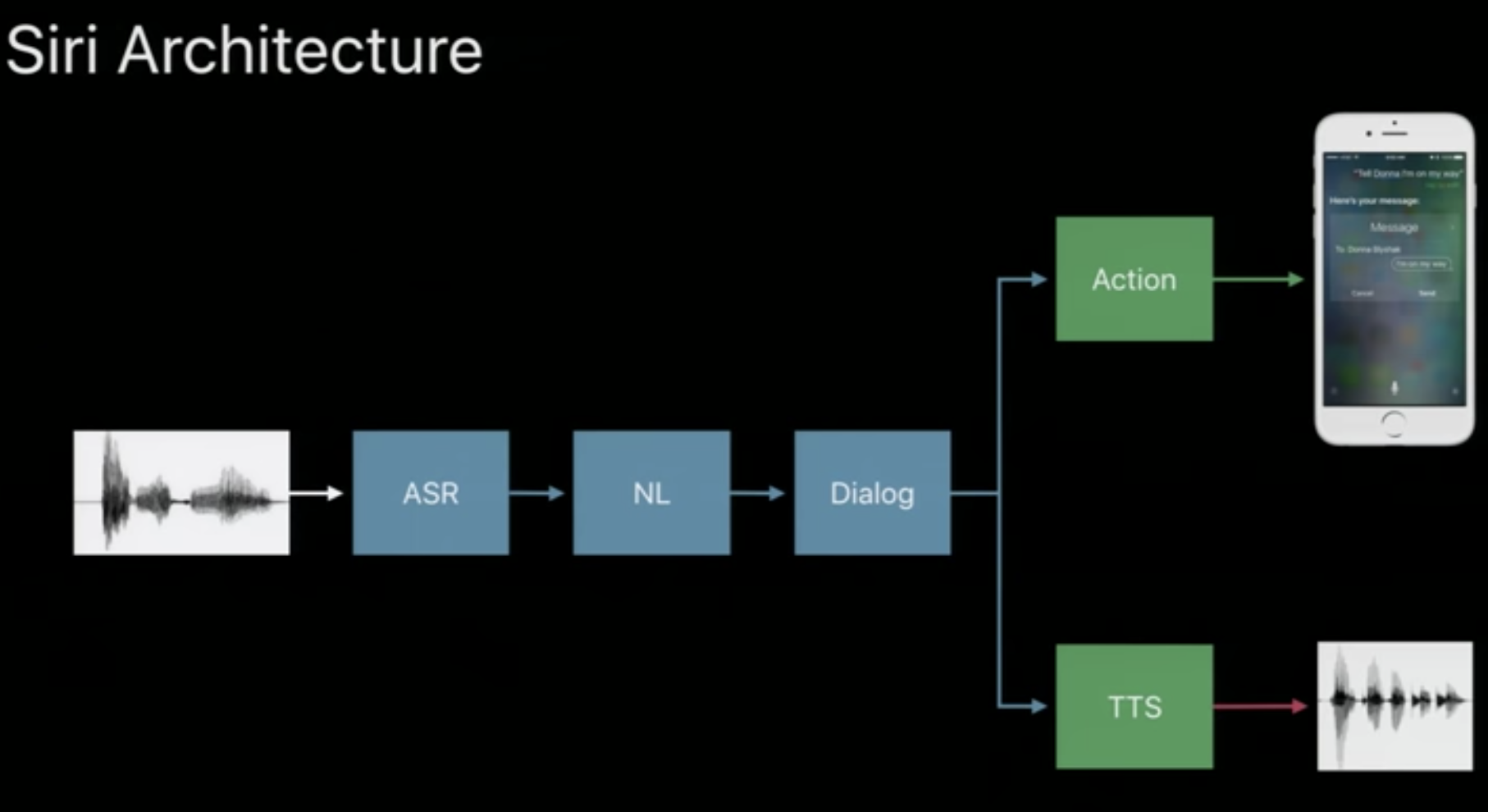
  - Start with a Wave Form
  - Pass the wave form through an ASR system
  - Then use a Natural Language Model to re-adjust the labels
  - Output Words
  - Based on the output, do some action or save the output, etc.
- “Hey Siri” DNN:
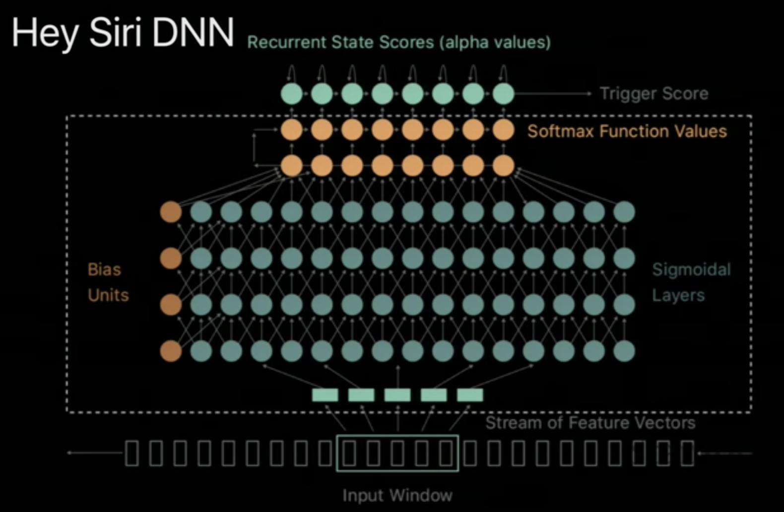
  - Much smaller DNN than for the full Vocab. ASR
  - Does Binary Classification - Did the speaker say “hey Siri” or not?
  - Consists of 5 Layers
  - The layers have few parameters
  - It has a Threshold at the end
  - So fast
  - Capable of running on the Apple Watch!
- Two-Pass Detection:
  - Problem:
    A big problem that arises in the always-on voice, is that it needs to run 24/7.
  - Solution:
    
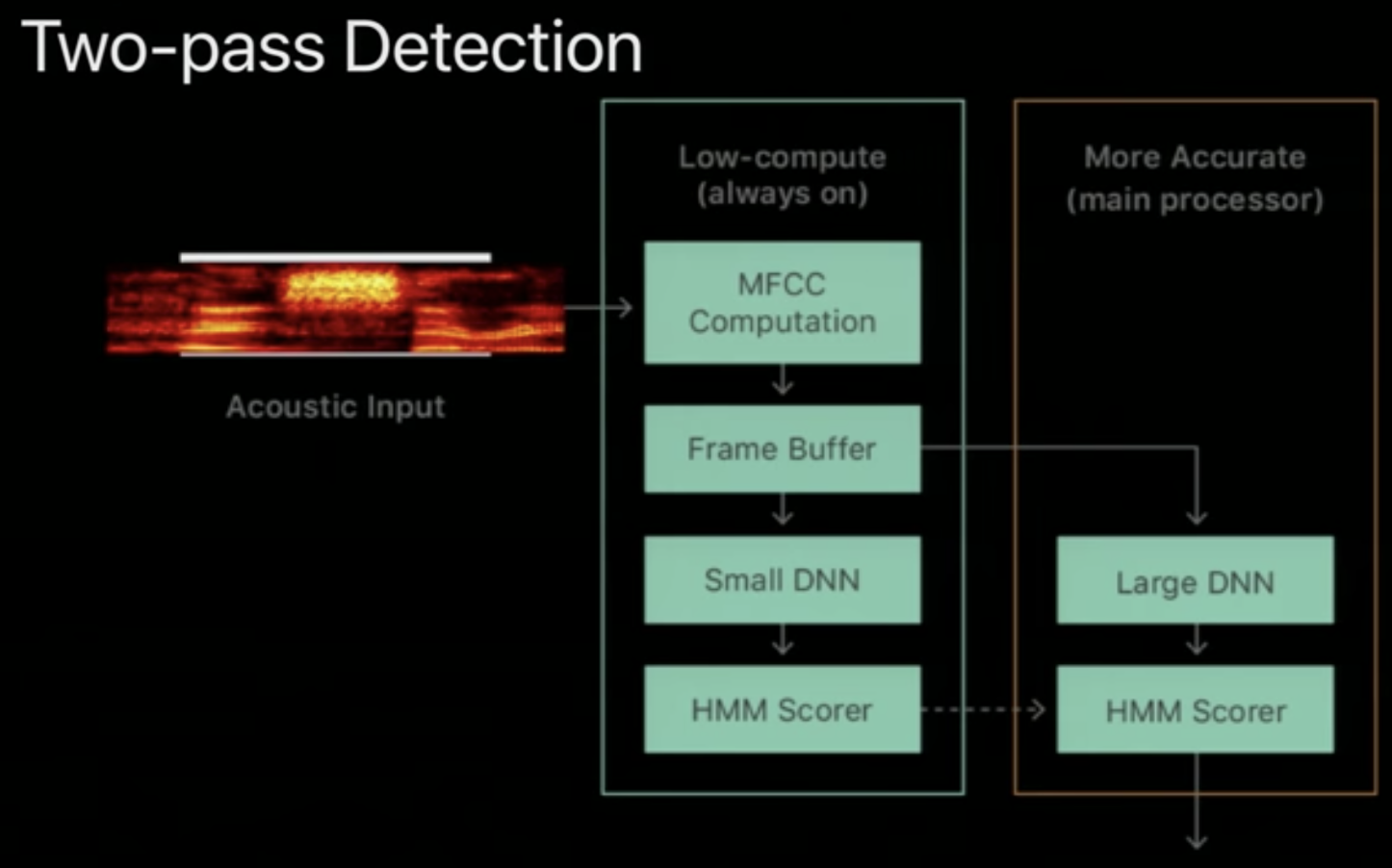
    We use a Two-Pass Detection system:
    
    There are two processors implemented in the phone:
    
    Low-Compute Processor:
    
    Always ON
    
    Given a threshold value of confidence over binary probabilities the Processor makes the following decision: “Should I wake up the Main Processor”
    
    Low power consumption
    
    Main Processor:
    
    Only ON if woken up by the low-compute processor
    
    Runs a much larger DNN
    
    High power consumption
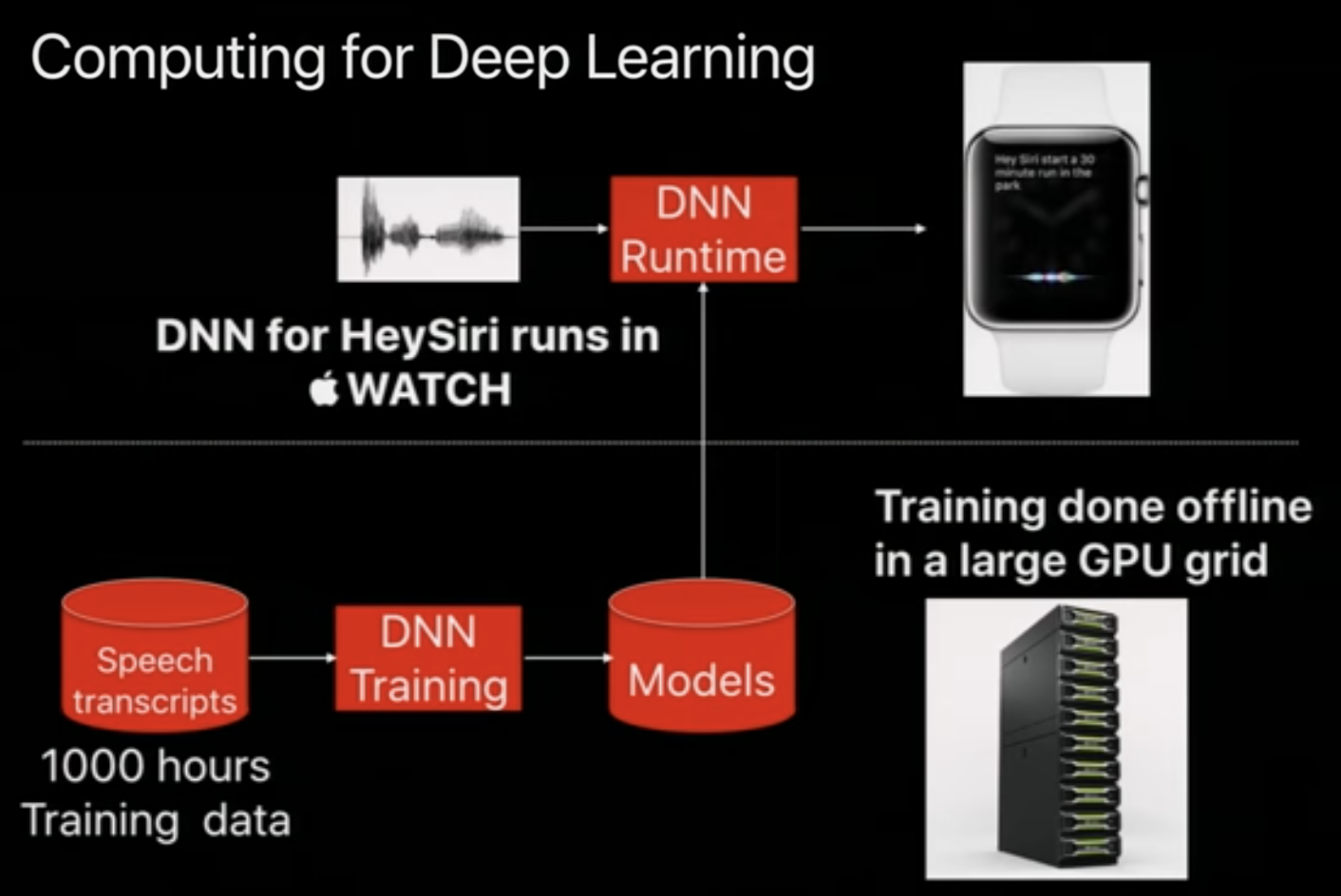
- Computation for DL:

Building ASR Systems

Pre-Processing:
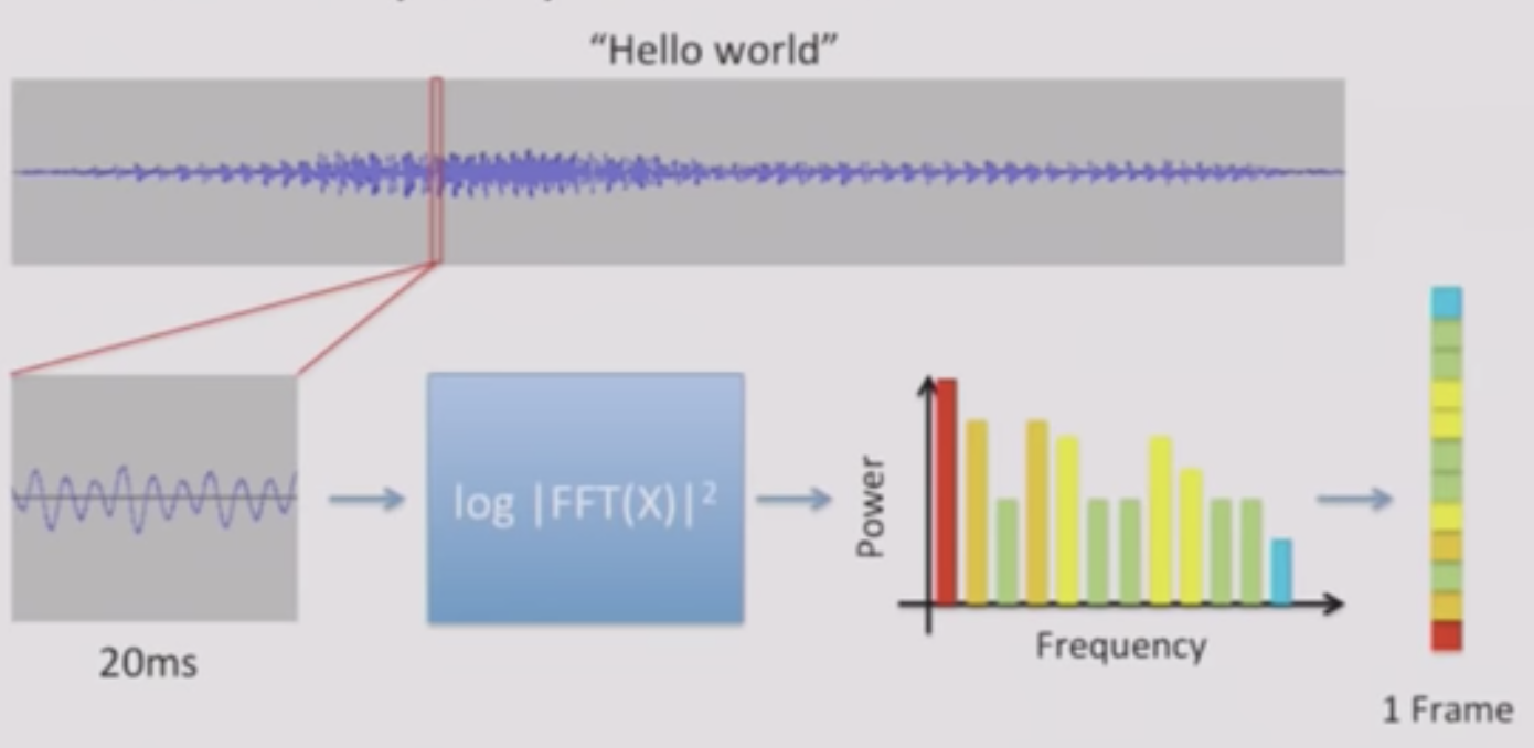
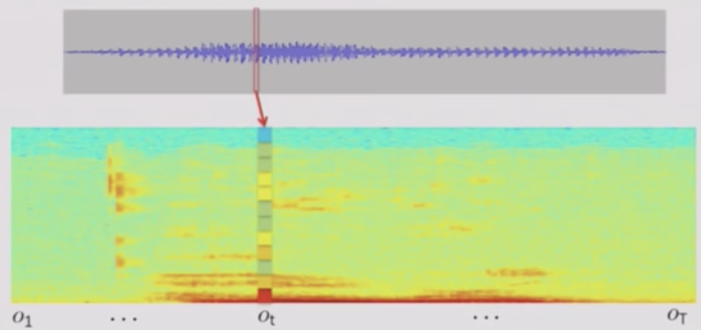
A Spectrogram is a visual representation of the spectrum of frequencies of sound or other signal as they vary with time.
- Take a small window (~20 ms) of waveform
- Compute FFT and take magnitude (i.e. prower)
  
  Describes Frequency content in local window
- Concatenate frames from adjacent windows to form the “spectrogram”
Acoustic Model:

An Acoustic Model is used in automatic speech recognition to represent the relationship between an audio signal and the phonemes or other linguistic units that make up speech.

Goal: create a neural network (DNN/RNN) from which we can extract transcriptions, $y$ - by training on labeled pairs $(x, y^\ast)$.
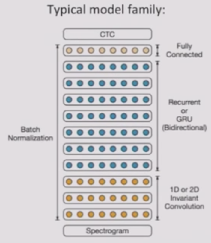
Network (example) Architecture:
RNN to predict graphemes (26 chars + space + blank):
- Spectrograms as inputs
- 1 Layer of Convolutional Filters
- 3 Layers of Gated Recurrent Units
  - 1000 Neurons per Layer
- 1 Fully-Connected Layer to predict $c$
- Batch Normalization
- CTC Loss Function (Warp-CTC)
- SGD+Nesterov Momentum Optimization/Training
Incorporating a Language Model:
Incorporating a Language Model helps the model learn:
- Spelling
- Grammar
- Expand Vocabulary
Two Ways:
1. Fuse the Acoustic Model with the language model $p(y)$
2. Incorporate linguistic data:
  - Predict Phonemes + Pronunciation Lexicon + LM
Decoding with Language Models:
- Given a word-based LM of form $p(w_{t+1} \vert w_{1:t})$
- Use Beam Search to maximize (Hannun et al. 2014):
\[\mathrm{arg } \max_{w} p(w \vert x)\: p(w)^\alpha \: [\text{length}(w)]^\beta\]
- $p(w \vert x) = p(y \vert x)$ for characters that make up $w$.
- We tend to penalize long transcriptions due to the multiplicative nature of the objective, so we trade off (re-weight) with $\alpha , \beta$
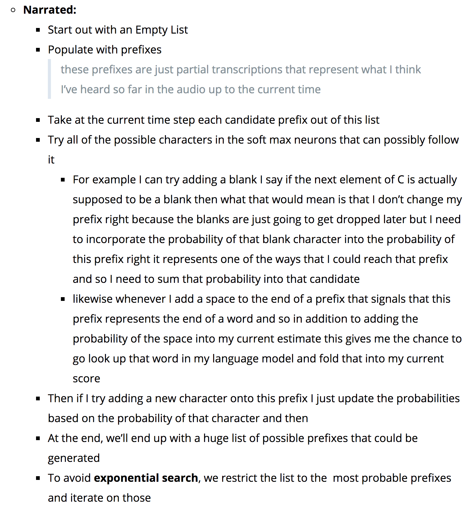
- Start with a set of candidate transcript prefixes, $A = {}$
- For $t = 1 \ldots T$:
  - For Each Candidate in $A$, consider:
    
    Add blank; don’t change prefix; update probability using the AM.
    
    Add space to prefix; update probability using LM.
    
    Add a character to prefix; update probability using AM. Add new candidates with updated probabilities to $A_{\text{new}}$
  - $A := K$ most probable prefixes in $A_{\text{new}}$
Rescoring with Neural LM:
The output from the RNN described above consists of a big list of the top $k$ transcriptions in terms of probability.
We want to re-score these probabilities based on a strong LM.
- It is Cheap to evaluate $p(w_k \vert w_{k-1}, w_{k-2}, \ldots, w_1)$ NLM on many sentences
- In-practice, often combine with N-gram trained from big corpora
Scaling Up:
- Data:
  - Transcribing speech data isn’t cheap, but not prohibitive
    
    Roughly 50¢ to $1 per minute
  - Typical speech benchmarks offer 100s to few 1000s of hours:
    
    LibriSpeech (audiobooks)
    
    LDC corpora (Fisher, Switchboard, WSJ) ($$)
    
    VoxForge
  - Data is very Application/Problem dependent and should be chosen with respect to the problem to be solved
  - Data can be collected as “read”-data for <$10 – Make sure the data to be read is scripts/plays to get a conversationalist response
  - Noise is additive and can be incorporated
- Computation:
  - How big is 1 experiment?{: style=”color: red”}
    $\geq (\# \text{Connections}) \cdot (\# \text{Frames}) \cdot (\# \text{Utterances}) \cdot (\# \text{Epochs}) \cdot 3 \cdot 2 \:\text{ FLOPs}$
    E.g. for DS2 with 10k hours of data:
    $100*10^6 * 100 * 10^6*20 * 3 * 2 = 1.2*10^{19} \:\text{ FLOPs}$
    ~30 days (with well-optimized code on Titan X)
  - Work-arounds and solutions:{: style=”color: red”}
    
    More GPUs with data parallelism:
    
    Minibatches up to 1024
    
    Aim for $\geq 64$ utterances per GPU ~$< 1$-wk training time (~8 Titans)
  - How to use more GPUs?{: style=”color: red”}
    
    Synch. SGD
    
    Asynch SGD
    
    Synch SGD w/ backup workers
  - Tips and Tricks:
    
    Make sure the code is optimized single-GPU.
    A lot of off-the-shelf code has inefficiencies.
    E.g. Watch for bad GEMM sizes.
    
    Keep similar-length utterances together:
    The input must be block-sized and will be padded; thus, keeping similar lengths together reduces unnecessary padding.
- Throughput:
  - Large DNN/RNN models run well on GPUs, ONLY, if the batch size is high enough.
    Processing 1 audio stream at a time is inefficient.
    Performance for K1200 GPU:
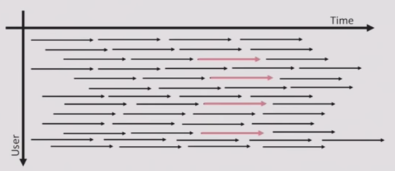
    | Batch Size | FLOPs | Throughput | | 1 | 0.065 TFLOPs | 1x | | 10 | 0.31 TFLOPs | 5x | | 32 | 0.92 TFLOPs | 14x |
  - Batch packets together as data comes in:
    
    Each packet (Arrow) of speech data ~ 100ms
    
    Process packets that arrive at similar times in parallel (from multiple users)

ASR
Automatic Speech Recognition

Table of Contents

Introduction to Speech

The Methods and Models of Speech Recognition

Transitioning into Deep Learning

Connectionist Temporal Classification

LAS - Seq2Seq with Attention

Online Seq2Seq Models

Real-World Applications

Building ASR Systems

ASR Automatic Speech Recognition

Table of Contents

Introduction to Speech

The Methods and Models of Speech Recognition

Transitioning into Deep Learning

Connectionist Temporal Classification

LAS - Seq2Seq with Attention

Online Seq2Seq Models

Real-World Applications

Building ASR Systems

ASR
Automatic Speech Recognition