Ahmad Badary

Introduction

Big Idea:

Express a numeric computation as a graph.
Main Components:
- Graph Nodes:
  are Operations which have any number of Inputs and Outputs
- Graph Edges:
  are Tensors which flow between nodes
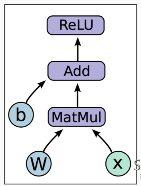
Example:

\(h = \text{ReLU}(Wx+b) \\ \rightarrow\)
Components of the Graph:
- Variables: are stateful nodes which output their current value.
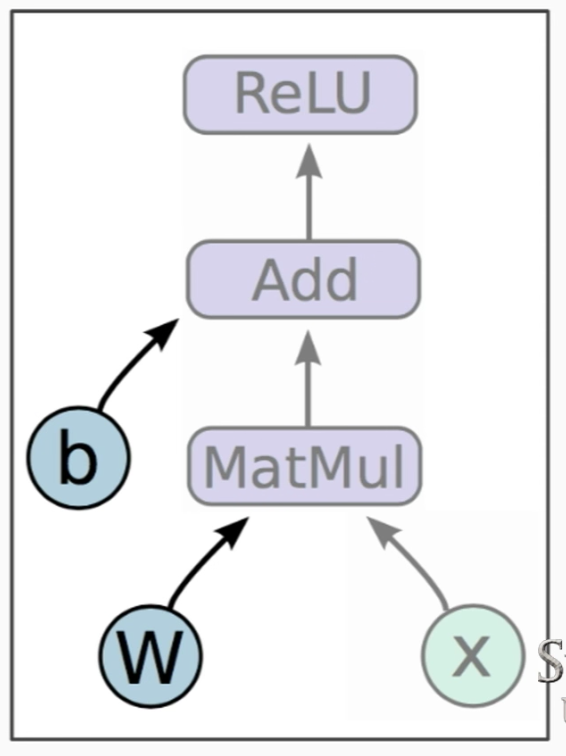
  - State is retained across multiple executions of a graph.
  - It is easy to restore saved values to variables
  - They can be saved to the disk, during and after training
  - Gradient updates, by default, will apply over all the variables in the graph
  - Variables are, still, by “definition” operations
  - They constitute mostly, Parameters
- Placeholders: are nodes whose value is fed in at execution time.
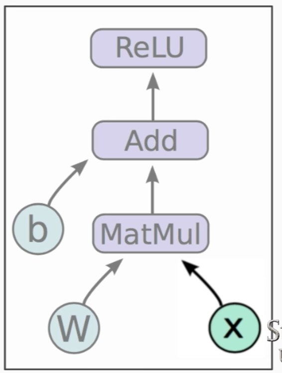
  - They do not have initial values
  - They are assigned a:
    
    data-type
    
    shape of a tensor
  - They constitute mostly, Inputs and labels
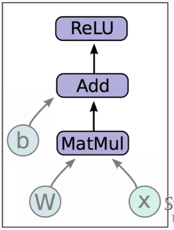
- Mathematical Operations:

Sample Code:

import tensorflow as tf
b = tf.Variable(tf.zeros((100,)))
W = tf.Variable(tf.random_uniform((784, 100) -1, 1))
x = tf.placeholder(tf.float32, (100, 784))  
h = tf.nn.relu(tf.matmul(x, W) + b)

Running the Graph:

After defining a graph, we can deploy the graph with a
Session: a binding to a particular execution context

i.e. the Execution Environment
- CPU
  or
- GPU
Getting the Output:
- Create the session object
- Run the session object on:
  - Fetches: List of graph nodes.
    Returns the outputs of these nodes.
  - Feeds: Dictionary mapping from graph nodes to concrete values.
    Specifies the value of each graph node given in the dictionary.
- CODE:
  sess = tf.Session() sess.run(tf.initialize_all_variables()) sess.run(h, {x: np.random.random(100, 784)})

Defining the Loss:

Use placeholder for labels
Build loss node using labels and prediction

CODE:

  prediction = tf.nn.softmax(...) # output of neural-net
  label = tf.placeholder(tf.float32, [100, 10])
  cross_entropy = -tf.reduce_sum(label * tf.log(prediction), axis=1)

Computing the Gradients:
- We have an Optimizer Object:
  tf.train.GradientDescentOptimizaer
- We, then, add Optimization Operation to computation graph:
  tf.train.GradientDescentOptimizer(lr).minimize(cross_entropy)
- CODE:
  train_step = tf.train.GradientDescentOptimizer(0.5).minimize(cross_entropy)

Training the Model:

sess = tf.Session()
sess.run(tf.initialize_all_variables())

for i in range(1000):
    batch_x, batch_label = data.next_batch()
    sess.run(train_step, feed_dict={x: batch_x, label: batch_label})  

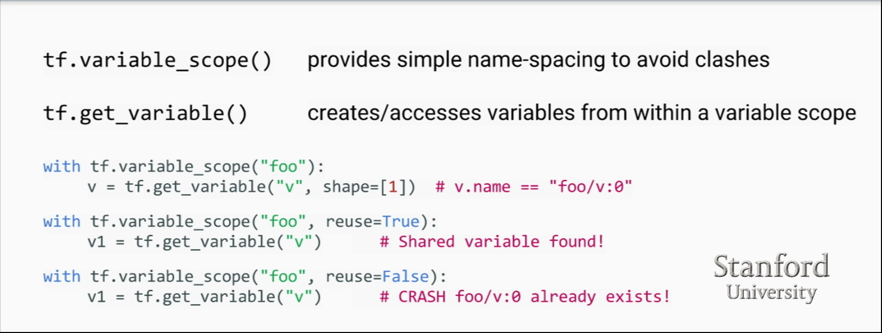
Variable Scope:

THIRD

Introduction and Definitions:
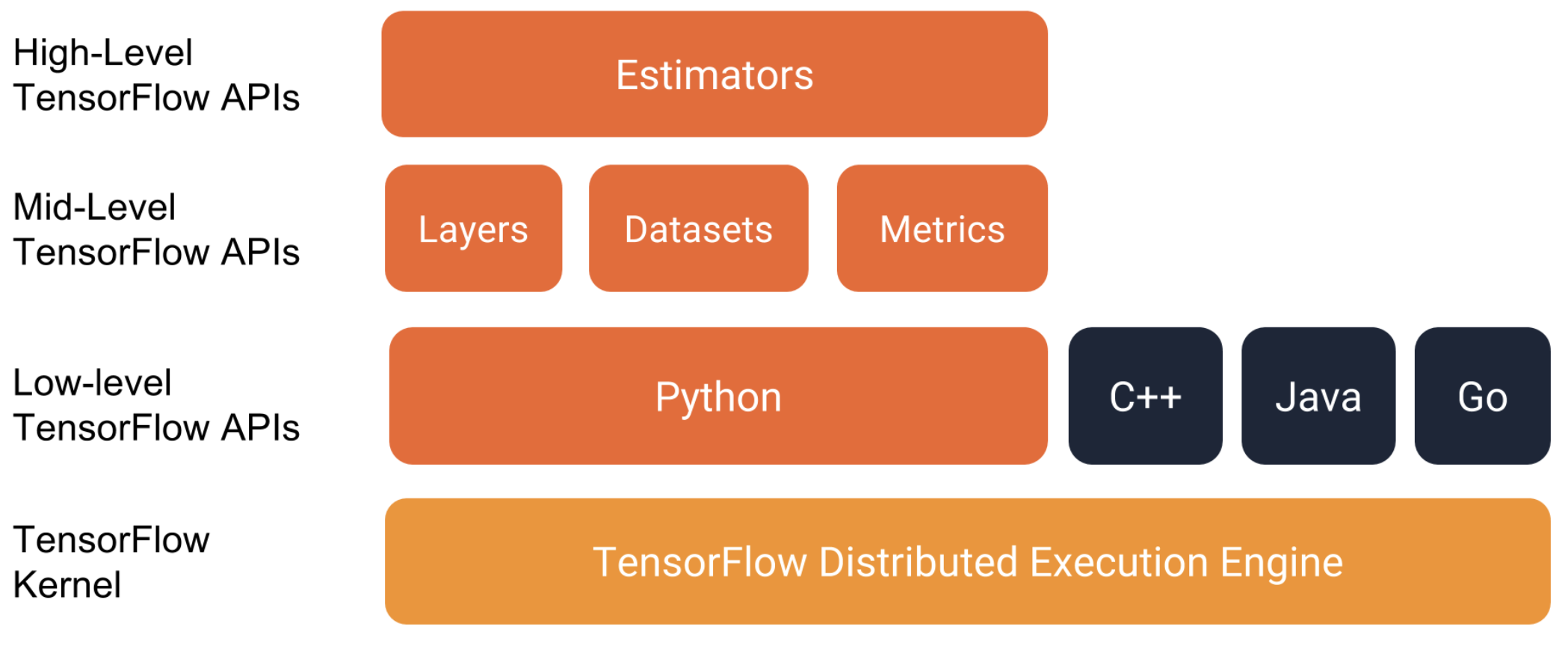
- Hierarchy:
- Input Function:
  An input function is a function that returns a tf.data.Dataset object which outputs the following two-element tuple:
  - features - A python dict in which:
    
    Each key is the name of a feature
    
    Each value is an array containing all of that features values
  - label - An array containing the values of the label for every example.
    def train_input_fn(features, labels, batch_size): """An input function for training""" # Convert the inputs to a Dataset. dataset = tf.data.Dataset.from_tensor_slices((dict(features), labels)) # Shuffle, repeat, and batch the examples. return dataset.shuffle(1000).repeat().batch(batch_size)

Import and Parse the data sets:

e.g. Iris DataSet with KERAS

TRAIN_URL = "http://download.tensorflow.org/data/iris_training.csv"
TEST_URL = "http://download.tensorflow.org/data/iris_test.csv"
# Train
train_path = tf.keras.utils.get_file(fname=TRAIN_URL.split('/')[-1], origin=TRAIN_URL)
train = pd.read_csv(filepath_or_buffer=train_path, names=CSV_COLUMN_NAMES)
train_features, train_label = train, train.pop(label_name)
# Test
test_path = tf.keras.utils.get_file(TEST_URL.split('/')[-1], TEST_URL)
test = pd.read_csv(test_path, names=CSV_COLUMN_NAMES, header=0)
test_features, test_label = test, test.pop(label_name)

Describe the data:

Creating features.
E.g. Numeric

my_feature_columns = []
for key in train_x.keys():
    my_feature_columns.append(tf.feature_column.numeric_column(key=key))

Select the type of model:

To specify a model type, instantiate an Estimator class:

Pre-made
Custom

E.g. DNNClassifier

classifier = tf.estimator.DNNClassifier(feature_columns=my_feature_columns, hidden_units=[10, 10], n_classes=3, optimizer='SGD')

Train the model:

Instantiating a tf.Estimator.DNNClassifier creates a framework for learning the model. Basically, we’ve wired a network but haven’t yet let data flow through it.

To train the neural network, call the Estimator object’s train method:
classifier.train( input_fn=lambda:train_input_fn(train_feature, train_label, args.batch_size), steps=args.train_steps)
- The steps argument tells train to stop training after the specified number of iterations.
- The input_fn parameter identifies the function that supplies the training data. The call to the train method indicates that the train_input_fn function will supply the training data with signature:
  def train_input_fn(features, labels, batch_size):
  The following call converts the input features and labels into a tf.data.Dataset object, which is the base class of the Dataset API:
  dataset = tf.data.Dataset.from_tensor_slices((dict(features), labels)) # Modifying the data dataset = dataset.shuffle(buffer_size=1000).repeat(count=None).batch(batch_size)
  Setting the buffer_size to a value larger than the number of examples (120) ensures that the data will be well shuffled
Evaluate the model:

To evaluate a model’s effectiveness, each Estimator provides an evaluate method:
# Evaluate the model. eval_result = classifier.evaluate( input_fn=lambda:eval_input_fn(test_x, test_y, args.batch_size)) print('\nTest set accuracy: {accuracy:0.3f}\n'.format(**eval_result))
The call to classifier.evaluate is similar to the call to classifier.train. The biggest difference is that classifier.evaluate must get its examples from the test set rather than the training set

Predicting:

Every Estimator provides a predict method, which premade_estimator.py calls as follows:

 predictions = classifier.predict(
 input_fn=lambda:eval_input_fn(predict_x,labels=None, batch_size=args.batch_size))

JIRA:
Project:
- A JIRA Project is a collection of issues
- Every issue belongs to a Project
- Each project is identified by a Name and Key
- Project Key is appended to each issue associated with the project
- Example:
  - Name of Project: Social Media Site
  - Project Key: SM
  - Issue: SM 24 Add a new friend
Issue:
- Issue is the building block of the project
- Depending on how your organization is using JIRA, an issue could represent:
  - a software bug
  - a project task
  - a helpdesk ticket
  - a product improvement
  - a leave request from client
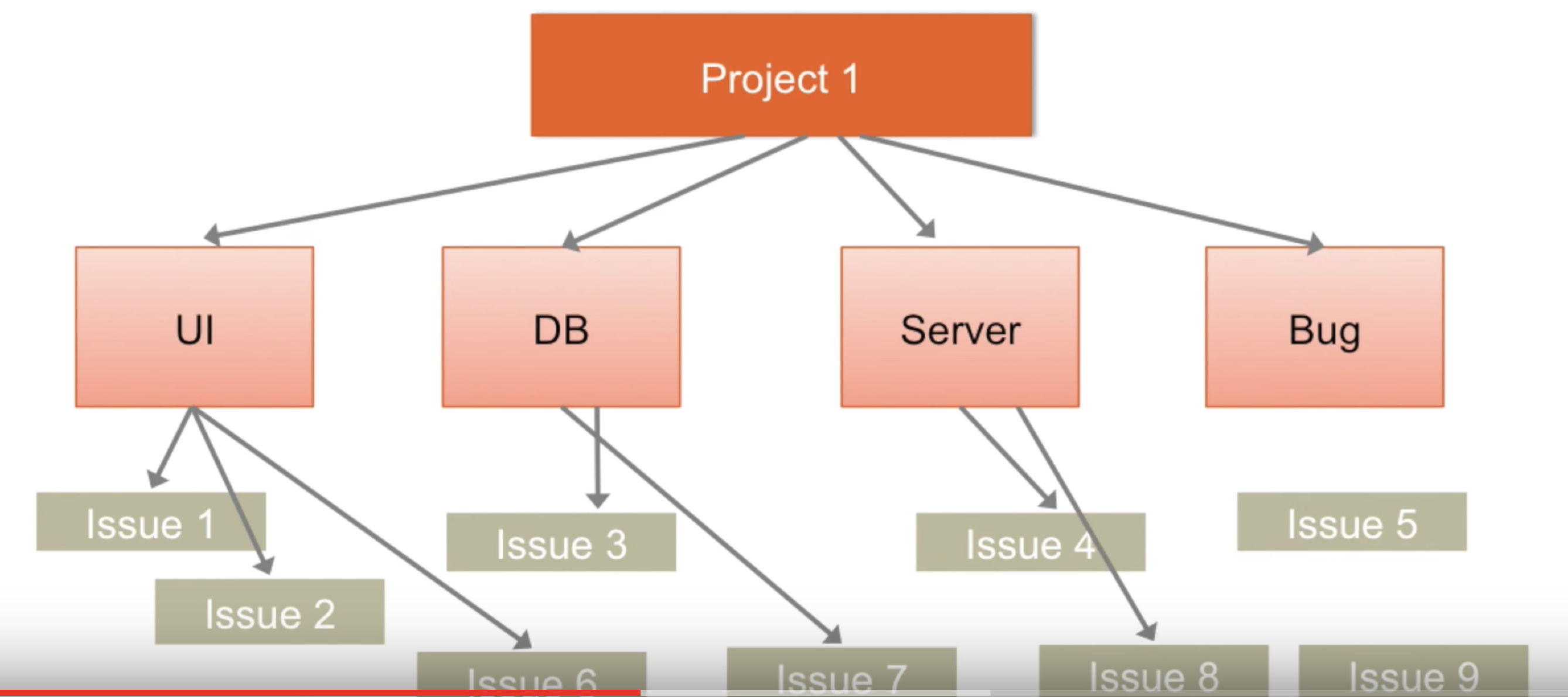
Components:
- Components are sub-sections of a project
- Components are used to group issues within a project to smaller parts
Workflow:
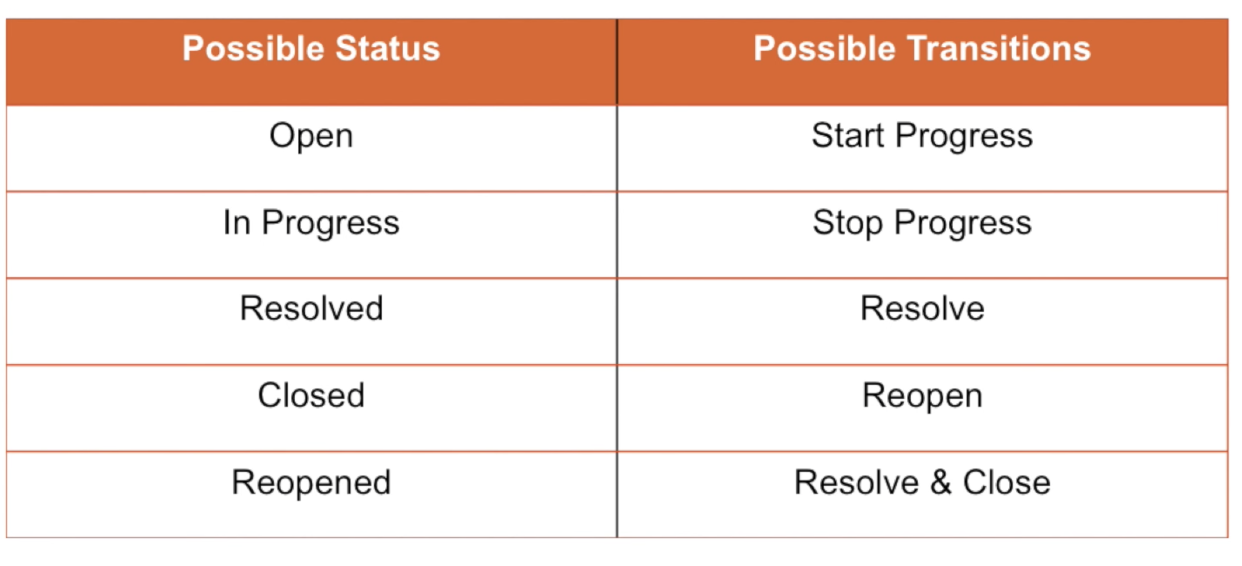
- A JIRA workflow is the set of statuses and transitions that an issue goes through during its lifecycle.
- Workflows typically represent business processes.
- JIRA comes with default workflow and it can be customized to fit your organization
Workflow Status and Transitions:

FOURTH

To write a TF program based on pre-made Estimator:
- Create one or more input function
- Define the models feature columns
- Instantiate an Estimator, specifying the feature columns and various hyperparameters.
- Call one or more methods on the Estimator object, passing the appropriate input function as the source of the data.

Checkpoint:

are saved automatically and are restored automatically after training.

Save by specifying which model_dir to save into:

classifier = tf.estimator.DNNClassifier(feature_columns=feature_columns, hidden_units=[10, 10], n_classes=3, model_dir='models/iris')

Feature Column:

check this page for the feature column functions

Custom Estimator:

Basically, you need to write a model function (model_fn) which implements the ML algo.

Write an Input Function (same)

Create feature columns (same)

Write a Model Function:

  def my_model_fn(
features, # This is batch_features from input_fn
labels,   # This is batch_labels from input_fn
mode,     # An instance of tf.estimator.ModeKeys
params):  # Additional configuration

The mode argument indicates whether the caller is requesting training, predicting, or evaluation.

Create the estimator:

  classifier = tf.estimator.Estimator(
 model_fn=my_model,
 params={
  'feature_columns': my_feature_columns,
  # Two hidden layers of 10 nodes each.
  'hidden_units': [10, 10],
  # The model must choose between 3 classes.
  'n_classes': 3,
 })

Writing Model Function:

You need to do:
- Define the Model
- Specify additional calculations:
  - Predict
  - Evaluate
  - Train
    
    Define the Model:
- The Input Layer:
  convert the feature dictionary and feature_columns into input for your model
```
      # Use `input_layer` to apply the feature columns.
 net = tf.feature_column.input_layer(features, params['feature_columns'])
```
- Hidden Layer:
  The Layers API provides a rich set of functions to define all types of hidden layers.
```
      # Build the hidden layers, sized according to the 'hidden_units' param.
 for units in params['hidden_units']:
  net = tf.layers.dense(net, units=units, activation=tf.nn.relu)
```
  The variable net here signifies the current top layer of the network. During the first iteration, net signifies the input layer.
  On each loop iteration tf.layers.dense creates a new layer, which takes the previous layer’s output as its input, using the variable net.
- Output Layer:
  Define the output layer by calling tf.layer.dense
```
  # Compute logits (1 per class).
 logits = tf.layers.dense(net, params['n_classes'], activation=None)
```
  When defining an output layer, the units parameter specifies the number of outputs. So, by setting units to params[‘n_classes’], the model produces one output value per class.
  Predict:
  # Compute predictions. predicted_classes = tf.argmax(logits, 1) if mode == tf.estimator.ModeKeys.PREDICT: predictions = { 'class_ids': predicted_classes[:, tf.newaxis], 'probabilities': tf.nn.softmax(logits), 'logits': logits, } return tf.estimator.EstimatorSpec(mode, predictions=predictions)
Embeddings:

An embedding is a mapping from discrete objects, such as words, to vectors of real numbers.
Saving Params:

```python saver = tf.train.Saver() # before ‘with’ saver.save(sess, ‘./checkpoints/generator.ckpt’) # After (within) first for-loop
To restore

saver.restore(sess, tf.train.latest_checkpoint(‘checkpoints’)) # after ‘with’

Complete Training Example (Low-Level)

Computational Graph:
- Operations: the nodes of the graph.
  They take in tensors and produce tensors.
- Tensors: the edges in the graph.
  They are the values flowing through the graph.
Tensorboard:
- First, save the computation graph to a tensorboard summary file:
writer = tf.summary.FileWriter('.') writer.add_graph(tf.get_default_graph())
This will produce an event file in the current directory.
- Launch Tensorboard:
  tensorboard --logdir
Session:

To evaluate tensors, instantiate a tf.Session object, informally known as a session.
A session encapsulates the state of the TensorFlow runtime, and runs TensorFlow operations.
- First, create a session:
  sess = tf.Session()
- Run the session:
  sess.run()
  It takes a dict of any tuples or any tensor.
  It evaluates the tensor.
Some TensorFlow functions return tf.Operations instead of tf.Tensors. The result of calling run on an Operation is None. You run an operation to cause a side-effect, not to retrieve a value. Examples of this include the initialization, and training ops demonstrated later.

Feeding:

x = tf.placeholder(tf.float32)
y = tf.placeholder(tf.float32)
z = x + y

print(sess.run(z, feed_dict={x: 3, y: 4.5}))
print(sess.run(z, feed_dict={x: [1, 3], y: [2, 4]}))

Datasets:

The preferred method of streaming data into a model instead of placeholders.

To get a runnable tf.Tensor from a Dataset you must first convert it to a tf.data.Iterator, and then call the Iterator’s get_next method.
Create the Iterator:
slices = tf.data.Dataset.from_tensor_slices(my_data) next_item = slices.make_one_shot_iterator().get_next() # Then pass as follows while True: try: print(sess.run(next_item)) except tf.errors.OutOfRangeError: break
If the Dataset depends on stateful operations (e.g. random value) you may need to initialize the iterator before using it, as shown below:
iterator = dataset.make_initializable_iterator() next_row = iterator.get_next()
Layers:

A trainable model must modify the values in the graph to get new outputs with the same input. Layers are the preferred way to add trainable parameters to a graph.

Layers package together both the variables and the operations that act on them.
The connection weights and biases are managed by the layer object.

E.g. a densely-connected layer performs a weighted sum across all inputs for each output and applies an optional activation function.
Creating Layers:
x = tf.placeholder(tf.float32, shape=[None, 3]) linear_model = tf.layers.Dense(units=1) y = linear_model(x)
Initializing Layers:
The layer contains variables that must be initialized before they can be used.
init = tf.global_variables_initializer() sess.run(init)
Executing Layers:
print(sess.run(y, {x: [[1, 2, 3],[4, 5, 6]]}))
Layer Function shortcuts:
For each layer class (like tf.layers.Dense) TensorFlow also supplies a shortcut function (like tf.layers.dense).
The only difference is that the shortcut function versions create and run the layer in a single call.
x = tf.placeholder(tf.float32, shape=[None, 3]) y = tf.layers.dense(x, units=1) # Is Equivalent to: x = tf.placeholder(tf.float32, shape=[None, 3]) linear_model = tf.layers.Dense(units=1) y = linear_model(x)
While convenient, this approach allows no access to the tf.layers.Layer object. This makes introspection and debugging more difficult, and layer reuse impossible.

Example:

x = tf.constant([[1], [2], [3], [4]], dtype=tf.float32)
y_true = tf.constant([[0], [-1], [-2], [-3]], dtype=tf.float32)

linear_model = tf.layers.Dense(units=1)

y_pred = linear_model(x)
loss = tf.losses.mean_squared_error(labels=y_true, predictions=y_pred)

optimizer = tf.train.GradientDescentOptimizer(0.01)
train = optimizer.minimize(loss)

init = tf.global_variables_initializer()

sess = tf.Session()
sess.run(init)
for i in range(5000):
  _, loss_value = sess.run((train, loss))
  print(loss_value)

print(sess.run(y_pred))

TensorFlow

Introduction

THIRD

FOURTH

To restore

Complete Training Example (Low-Level)