W2V Detailed Tutorial - Skip Gram (Stanford)
W2V Detailed Tutorial - Negative Sampling (Stanford)
Commented word2vec C code
W2V Resources
An overview of word embeddings and their connection to distributional semantic models
On Word Embeddings (Ruder)

• Eigenwords: Spectral Word Embeddings (paper!)
• Stop Using word2vec (blog)
• Word2vec Inspired Recommendations In Production (blog)

Word Meaning

1. Representing the Meaning of a Word:
   Commonest linguistic way of thinking of meaning:
   Signifier \(\iff\) Signified (idea or thing) = denotation

2. How do we have usable meaning in a computer:
   Commonly: Use a taxonomy like WordNet that has hypernyms (is-a) relationships and synonym sets

3. Problems with this discrete representation:
   • Great as a resource but missing nuances:
     • Synonyms:
       adept, expert, good, practiced, proficient, skillful
   • Missing New Words
   • Subjective
   • Requires human labor to create and adapt
   • Hard to compute accurate word similarity:
     • One-Hot Encoding: in vector space terms, this is a vector with one 1 (at the position of the word) and a lot of zeroes (elsewhere).
       • It is a localist representation
       • There is no natural notion of similarity in a set of one-hot vectors

4. Distributed Representations of Words:
   A method where vectors encode the similarity between the words.

   The meaning is represented with real-valued numbers and is “smeared” across the vector.

   Contrast with one-hot encoding.

5. Distributional Similarity:
   is an idea/hypothesis that one can describe the meaning of words by the context in which they appear in.

   Contrast with Denotational Meaning of words.

6. The Big Idea:
   We will build a dense vector for each word type, chosen so that it is good at predicting other words appearing in its context.

7. Learning Neural Network Word Embeddings:
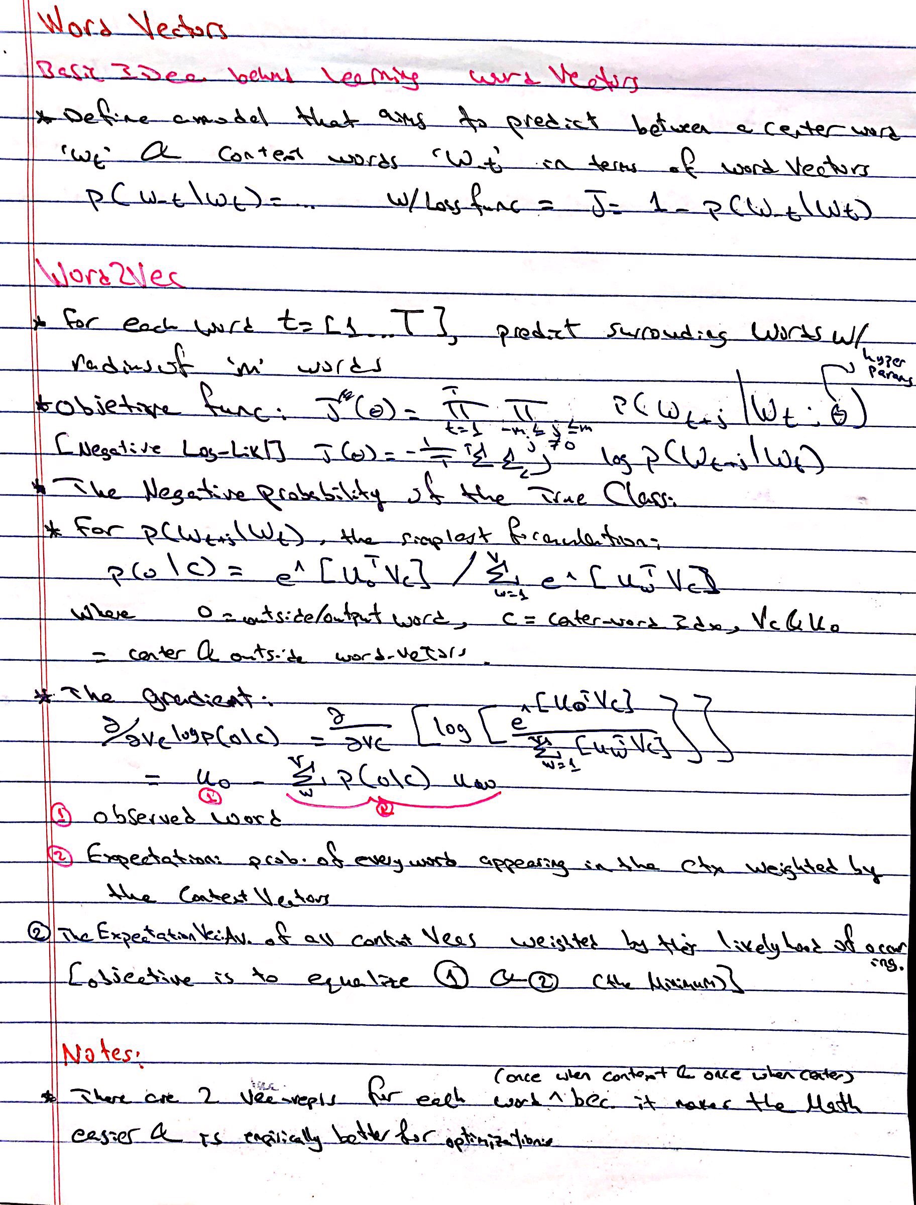
   We define a model that aims to predict between a center word \(w_t\) and context words in terms of word vectors.

   $$p(\text{context} \vert w_t) = \ldots$$

   The Loss Function:

   $$J = 1 - p(w_{-t} \vert w_t)$$

   We look at many positions \(t\) in a big language corpus
   We keep adjusting the vector representations of words to minimize this loss

8. Relevant Papers:
   • Learning representations by back-propagating errors (Rumelhart et al., 1986)
   • A neural probabilistic language model (Bengio et al., 2003)
   • NLP (almost) from Scratch (Collobert & Weston, 2008)
   • A recent, even simpler and faster model: word2vec (Mikolov et al. 2013) à intro now

Word Embeddings

1. Main Ideas:
   • Words are represented as vectors of real numbers
   • Words with similar vectors are semantically similar
   • Sometimes vectors are low-dimensional compared to the vocabulary size
2. The Clusterings:
   Relationships (attributes) Captured:
   • Synonyms: car, auto
   • Antonyms: agree, disagree
   • Values-on-a-scale: hot, warm, cold
   • Hyponym-Hypernym: “Truck” is a type of “car”, “dog” is a type of “pet”
   • Co-Hyponyms: “cat”&”dog” is a type of “pet”
   • Context: (Drink, Eat), (Talk, Listen)

3. Word Embeddings Theory:
   Distributional Similarity Hypothesis

4. History and Terminology:
   Word Embeddings = Distributional Semantic Model = Distributed Representation = Semantic Vector Space = Vector Space Model

5. Applications:
   • Word Similarity
   • Word Grouping
   • Features in Text-Classification
   • Document Clustering
   • NLP:
     • POS-Tagging
     • Semantic Analysis
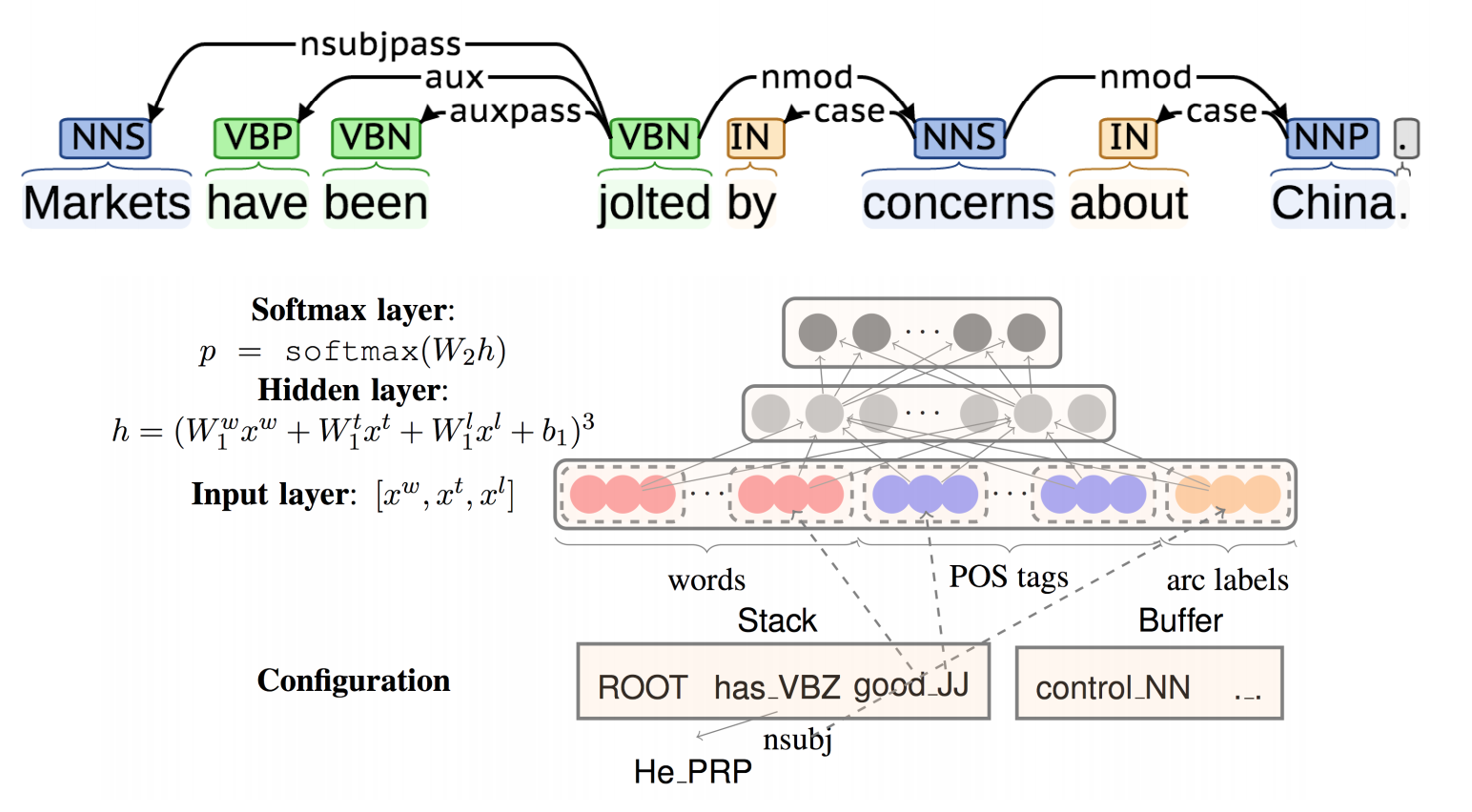
     • Syntactic Parsing
6. Approaches:
   • Count: word count/context co-occurrences
     • Distributional Semantics:
       1. Summarize the occurrence statistics for each word in a large document set:
          
       2. Apply some dimensionality reduction transformation (SVD) to the counts to obtain dense real-valued vectors:
          
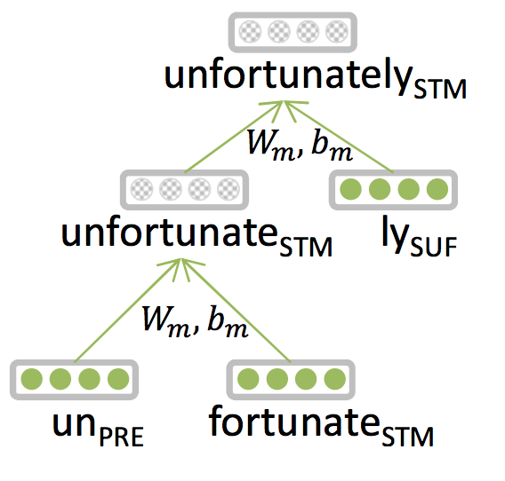
       3. Compute similarity between words as vector similarity:
          
   • Predict: word based on context
     • word2vec:
       1. In one setup, the goal is to predict a word given its context.
          
       2. Update word representations for each context in the data set
       3. Similar words would be predicted by similar contexts
7. Parameters:
   • Underlying Document Set
   • Context Size
   • Context Type
8. Software:
   

Word2Vec

1. Word2Vec:
   Word2Vec (Mikolov et al. 2013) is a framework for learning word representations as vectors. It is based on the idea of distributional similarity.
   
   

2. Main Idea:
   • Given a large corpus of text
   • Represent every word, in a fixed vocabulary, by a vector
   • Go through each position \(t\) in the text, which has a center word \(c\) and context words \(o\)
   • Use the similarity of the word vectors for \(c\) and \(o\) to calculate the probability of \(o\) given \(c\) (SG)
   • Keep adjusting the word vectors to maximize this probability

   

3. Algorithms:
   1. Skip-grams (SG):
      Predict context words given target (position independent)
   2. Continuous Bag of Words (CBOW):
      Predict target word from bag-of-words context
      
      
4. Training Methods:
   • Basic:
     1. Naive Softmax
   • (Moderately) Efficient:
     1. Hierarchical Softmax
     2. Negative Sampling
        
        
5. Skip-Gram Prediction Method:
   Skip-Gram Models aim to predict the distribution (probability) of context words from a center word.

   CBOW does the opposite, and aims to predict a center word from the surrounding context in terms of word vectors.

   The Algorithm:

   1. We generate our one hot input vector \(x \in \mathbf{R}^{\vert V\vert }\) of the center word.
   2. We get our embedded word vector for the center word \(v_c = V_x \in \mathbf{R}^n\)
   3. Generate a score vector \(z = \mathcal{U}_ {v_c}\)
   4. Turn the score vector into probabilities, \(\hat{y} = \text{softmax}(z)\)

      Note that \(\hat{y}_{c−m}, \ldots, \hat{y}_{c−1}, \hat{y}_{c+1}, \ldots, \hat{y}_{c+m}\) are the probabilities of observing each context word.

   5. We desire our probability vector generated to match the true probabilities, which is
      \(y^{(c−m)} , \ldots, y^{(c−1)} , y^{(c+1)} , \ldots, y^{(c+m)}\),
      the one hot vectors of the actual output.
      
      
6. Word2Vec Details:
   • For each word (position) \(t = 1 \ldots T\), predict surrounding (context) words in a window of “radius” \(m\) of every word.

   Calculating \(p(o \vert c)\)¹ the probability of outside words given center word:

   • We use two vectors per word \(w\):
     • \(v_{w}\): \(\:\) when \(w\) is a center word
     • \(u_{w}\): \(\:\) when \(w\) is a context word
   • Now, for a center word \(c\) and a context word \(o\), we calculate the probability:

     $$\\{\displaystyle p(o \vert c) = \dfrac{e^{u_o^Tv_c}}{\sum_{w\in V} e^{u_w^Tv_c}}} \:\:\:\:\:\:\:\:\:\:\:\:\\$$

     Constructing the Probability Distribution (Prediction Function)

     
     

7. The Objective:
   Goal:
   Maximize the probability of any context word given the current center word.

   We start with the Likelihood of being able to predict the context words given center words and the parameters \(\theta\) (only the wordvectors).
   The Likelihood:

   $$L(\theta)=\prod_{t=1}^{T} \prod_{-m \leq j \leq m \atop j \neq 0} P\left(w_{t+j} | w_{t} ; \theta\right)$$

   The objective:
   The Objective is just the (average) negative log likelihood:

   $$J(\theta) = -\frac{1}{T} \log L(\theta)= - \dfrac{1}{T} \sum_{t=1}^{t} \sum_{-m \leq j \leq m \\ \:\:\:\:j\neq 0} \log p(w_{t+j} \vert w_t ; \theta))$$

   Notice: Minimizing objective function \(\iff\) Maximizing predictive accuracy²
   
   

8. The Gradients:
   We have a vector of parameters \(\theta\) that we are trying to optimize over, and We need to calculate the gradient of the two sets of parameters in \(\theta\); namely, \(\dfrac{\partial}{\partial v_c}\) and \(\dfrac{\partial}{\partial u_o}\).

   The gradient \(\dfrac{\partial}{\partial v_c}\):

   $$\dfrac{\partial}{\partial v_c} \log p(o\vert c) = u_o - \sum_{w'\in V} p{(w' | c)} \cdot u_{w'}$$

   Interpretation:
   We are getting the slope by: taking the observed representation of the context word and subtracting away (“what the model thinks the context should look like”) the weighted average of the representations of each word multiplied by its probability in the current model
   (i.e. the Expectation of the context word vector i.e. the expected context word according to our current model)

   I.E.
   The difference between the expected context word and the actual context word

   Importance Sampling:

   $$\sum_{w_{i} \in V} \left[\frac{\exp \left(-\mathcal{E}\left(w_{i}\right)\right)}{\sum_{w_{i} \in V} \exp \left(-\mathcal{E}\left(w_{i}\right)\right)}\right] \nabla_{\theta} \mathcal{E}\left(w_{i}\right) \\ = \sum_{w_{i} \in V} P\left(w_{i}\right) \nabla_{\theta} \mathcal{E}\left(w_{i}\right)$$

   
   

   $$\mathbb{E}_{w_{i} \sim P}\left[\nabla_{\theta} \mathcal{E}\left(w_{i}\right)\right] =\sum_{w_{i} \in V} P\left(w_{i}\right) \nabla_{\theta} \mathcal{E}\left(w_{i}\right)$$

   • \(P\left(w_{i}\right) \approx \frac{r(w_i)}{R}\),

   $$\mathbb{E}_{w_{i} \sim P}\left[\nabla_{\theta} \mathcal{E}\left(w_{i}\right)\right] \approx \sum_{w_{i} \in V} \frac{r(w_i)}{R} \nabla_{\theta} \mathcal{E}\left(w_{i}\right)$$

   $$\mathbb{E}_{w_{i} \sim P}\left[\nabla_{\theta} \mathcal{E}\left(w_{i}\right)\right] \approx \frac{1}{R} \sum_{i=1}^{m} r\left(w_{i}\right) \nabla_{\theta} \mathcal{E}\left(w_{i}\right)$$

   where \(r(w)=\frac{\exp (-\mathcal{E}(w))}{Q(w)}\), \(R=\sum_{j=1}^{m} r\left(w_{j}\right)\), and \(Q\) is the unigram distribution of the training set.

9. Notes:
   • Mikolov on SkipGram vs CBOW:
     • Skip-gram: works well with small amount of the training data, represents well even rare words or phrases.
     • CBOW: several times faster to train than the skip-gram, slightly better accuracy for the frequent words.
   • Further Readings:
     • A Latent Variable Model Approach to PMI-based Word Embeddings
     • Linear Algebraic Structure of Word Senses, with Applications to Polysemy
     • On the Dimensionality of Word Embedding
     • Improving Distributional Similarity with Lessons Learned from Word Embeddings

• From ‘concepts’:
  Word Vectors:
  • Learning Word Vectors and Word2Vec
  • Word Vectors and Polysemy

  Notes:

  • Categorization is a method for Evaluating w2v Embeddings by creating categorize by clustering, then measuring the purity of the clusters

Notes:

• Word2vec maximizes the objective by putting similar words close to each other in space

• pictures from lecture:
  w2v:
  

  Softmax:
  

  Training/Optimization:
  

  Optimization - GD:
  

    GD
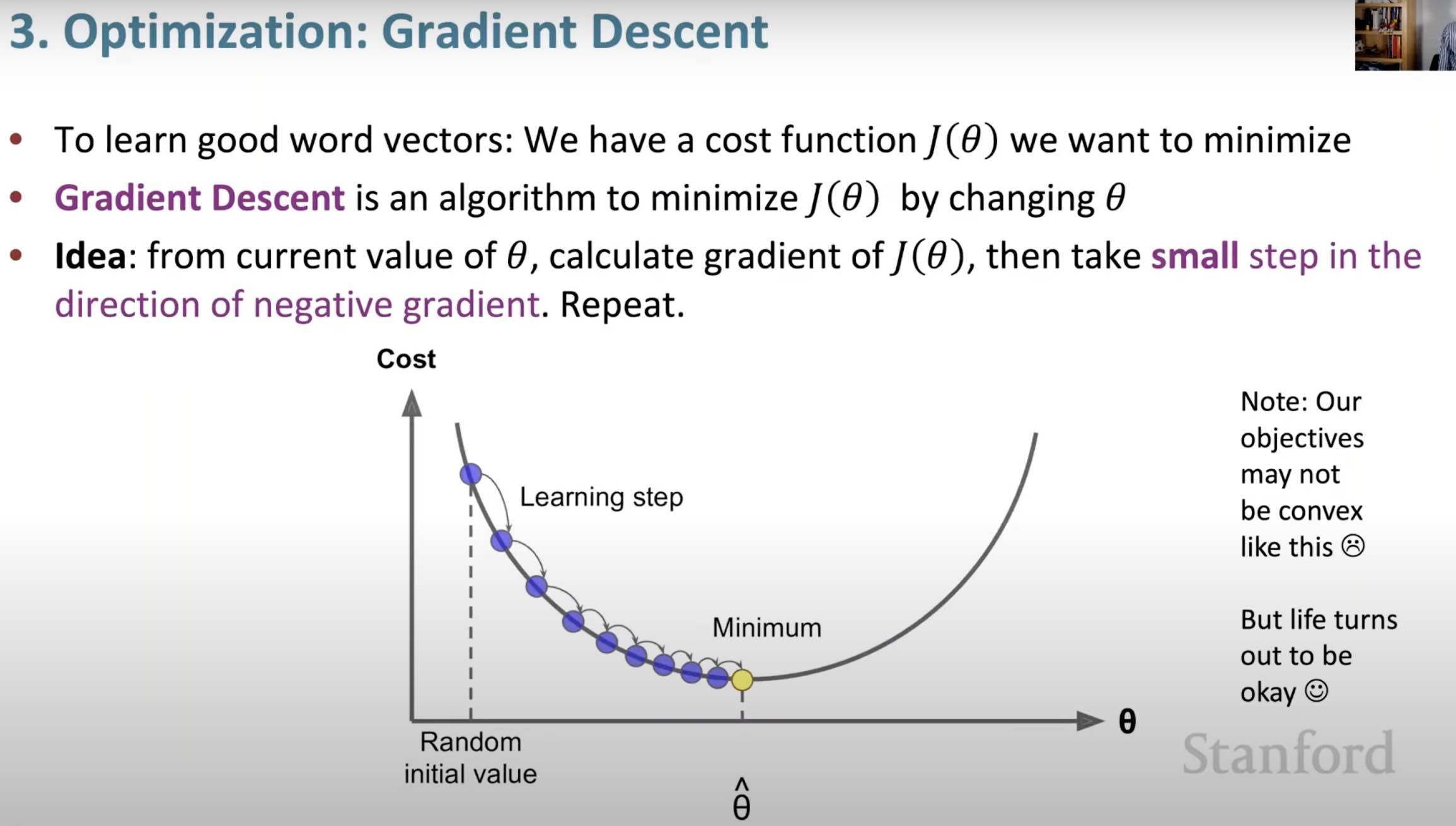
    ![img](https://cdn.mathpix.com/snip/images/L7qtJIlEs4StLvX-GJL6PKsUGQQJB4YCgIIxzYwxgfM.original.fullsize.png){: width="80%"}  
  
    SGD: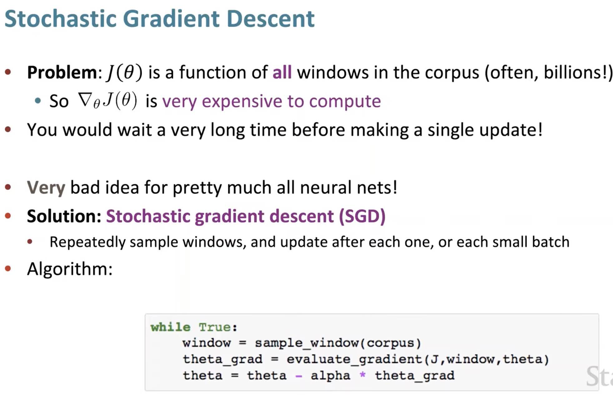  
    ![img](https://cdn.mathpix.com/snip/images/9rpsoP8b_iWjln2LNvVQC15kbtz2UF92hZlFbxlgy_Q.original.fullsize.png){: width="80%"}  
  
    <button>SGD</button>{: .showText value="show" onclick="showTextPopHide(event);"}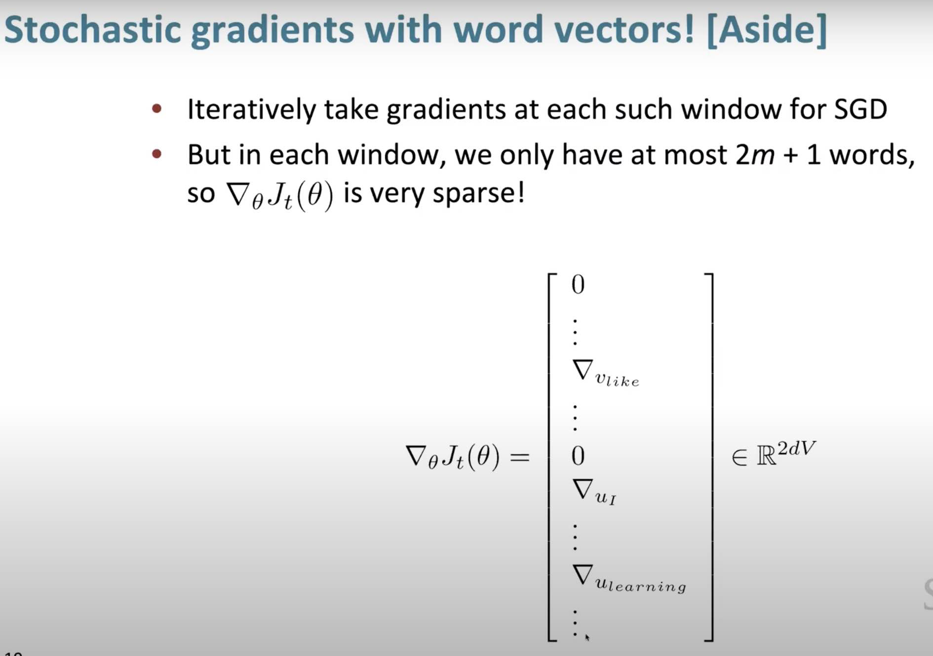
    ![img](https://cdn.mathpix.com/snip/images/8gsRPhIgUpvNtGPSYeQm03D0H_v-9_AzvcvjNp2OHqo.original.fullsize.png){: width="100%" hidden=""}  
  
    <button>SGD</button>{: .showText value="show" onclick="showTextPopHide(event);"}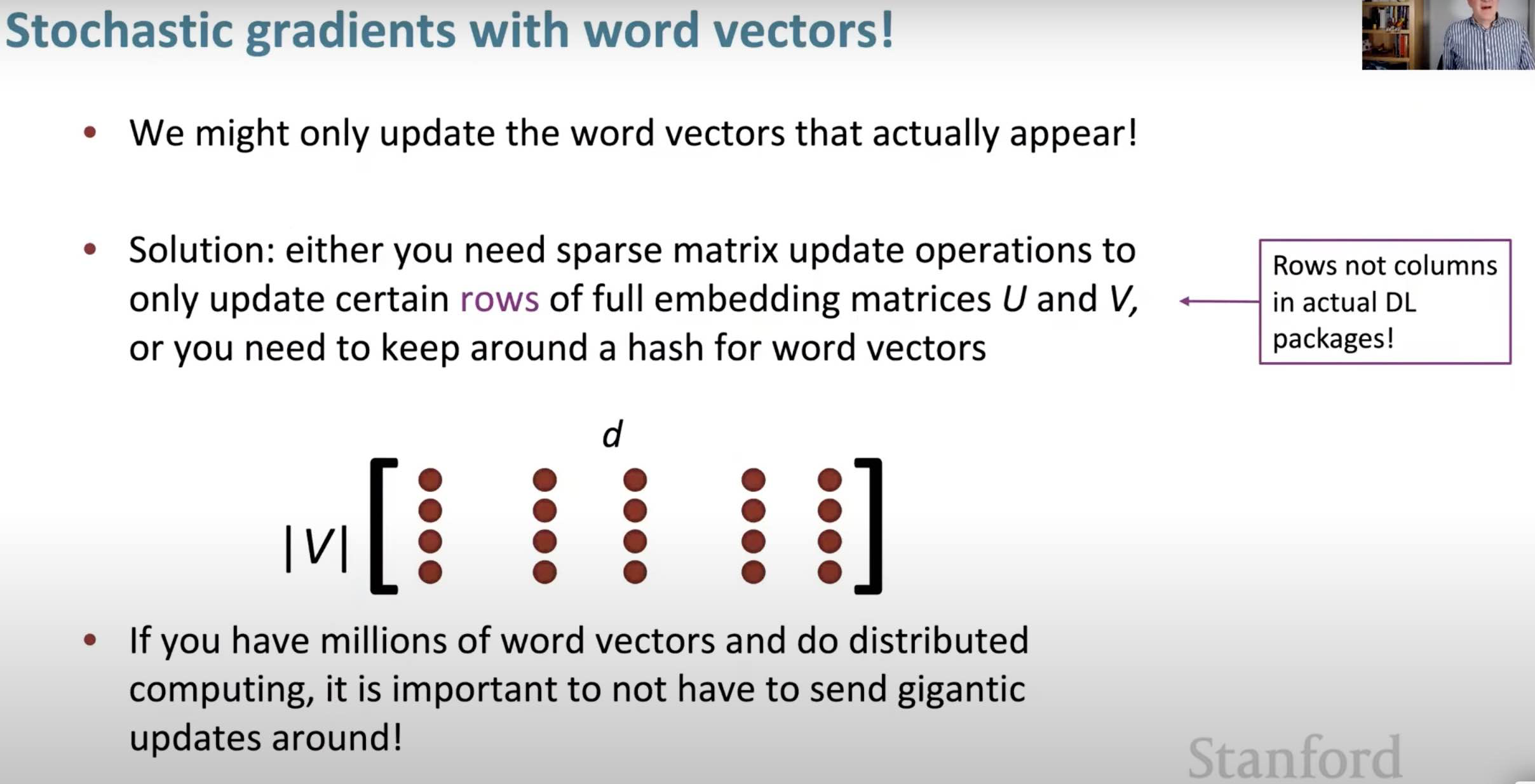
    ![img](https://cdn.mathpix.com/snip/images/_e3VK3CbGswucKUcjKFG9cpxFFBpxatSqasKFFfL6Nc.original.fullsize.png){: width="100%" hidden=""}  
    Note: rows can be accessed as a _contiguous block in memory_ (so if row is a word, you can access it much more efficiently)  
  

  W2V Algorithm Family

  Negative Sampling

  Skip-gram with NS - Paper Notation (maximize \(J\))

  Skip-gram with NS - Stanford Notation (minimize \(J\))

  • Unigram Distribution: A distribution of words based on how many times each word appeared in a corpus is called unigram distribution.
    Unigram Distribution and smoothing

  • Noise Distribution:

    • Noise Distribution (Blog)

  • Relevant stackOF Question

  • Optimize Computational Efficiency of Skip-Gram with Negative Sampling (Blog)

  • Demystifying Neural Network in Skip-Gram Language Modeling (Blog!!!!)

  • Understanding Multi-Dimensionality in Vector Space Modeling (Blog!!)