Table of Contents
Semantic Segmentation
-
- Semantic Segmentation:
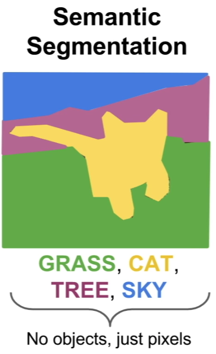
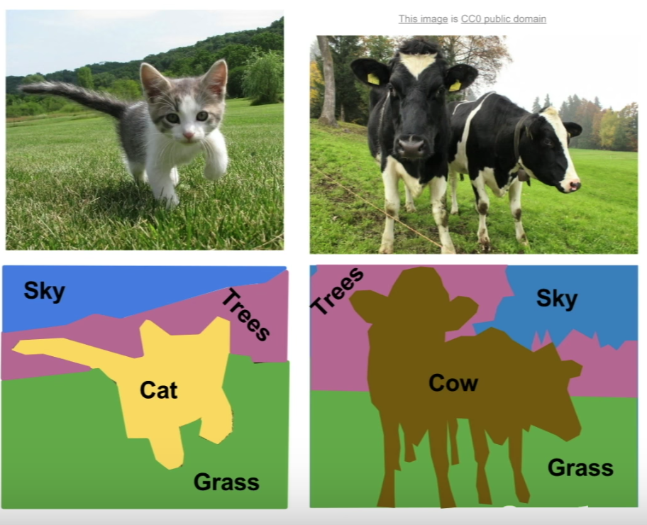
- Semantic Segmentation is the task of understanding an image at the pixel level. It seeks to assign an object class to each pixel in the image.
-
- The Structure:
-
- Input: Image
- Output: A class for each pixel in the image.
-
- Properties:
- In Semantic Segmentation, we don’t differentiate among the instances, instead, we only care about the pixels.
Approaches (The Pre-DeepLearning Era)
-
- Semantic Texton Forests:
- This approach consists of ensembles of decision trees that act directly on image pixels.
- Semantic Texton Forests (STFs) are randomized decision forests that use only simple pixel comparisons on local image patches, performing both an implicit hierarchical clustering into semantic textons and an explicit local classification of the patch category.
- STFs allow us to build powerful texton codebooks without computing expensive filter-banks or descriptors, and without performing costly k-means clustering and nearest-neighbor assignment.
- Semantic Texton Forests for Image Categorization and Segmentation, Shawton et al. (2008)
-
- Random Forest-based Classifiers:
- Random Forests have also been used to perform semantic segmentation for a variety of tasks.
-
- Conditional Random Fields:
- CRFs provide a probabilistic framework for labeling and segmenting structured data.
- They try to model the relationship between pixels, e.g.:
- nearby pixels more likely to have same label
- pixels with similar color more likely to have same label
- the pixels above the pixels “chair” more likely to be “person” instead of “plane”
- refine results by iterations
- W. Wu, A. Y. C. Chen, L. Zhao and J. J. Corso (2014): “Brain Tumor detection and segmentation in a CRF framework with pixel-pairwise affinity and super pixel-level features”
- Plath et al. (2009): “Multi-class image segmentation using conditional random fields and global classification”
-
- SuperPixel Segmentation:
- The concept of superpixels was first introduced by Xiaofeng Ren and Jitendra Malik in 2003.
- Superpixel is a group of connected pixels with similar colors or gray levels.
They produce an image patch which is better aligned with intensity edges than a rectangular patch. - Superpixel segmentation is the idea of dividing an image into hundreds of non-overlapping superpixels.
Then, these can be fed into a segmentation algorithm, such as Conditional Random Fields or Graph Cuts, for the purpose of segmentation. - Efficient graph-based image segmentation, Felzenszwalb, P.F. and Huttenlocher, D.P. International Journal of Computer Vision, 2004
- Quick shift and kernel methods for mode seeking, Vedaldi, A. and Soatto, S. European Conference on Computer Vision, 2008
- Peer Neubert & Peter Protzel (2014). Compact Watershed and Preemptive
Approaches (The Deep Learning Era)
-
- The Sliding Window Approach:
- We utilize classification for segmentation purposes.
-
- Algorithm:
- We break up the input image into tiny “crops” of the input image.
- Use Classification to find the class of the center pixel of the crop.
Using the same machinery for classification.
- Algorithm:
- Basically, we do classification on each crop of the image.
-
- DrawBacks:
- Very Inefficient and Expensive:
To label every pixel in the image, we need a separate “crop” for each pixel in the image, which would be quite a huge number. - Disregarding Localized Information:
This approach does not make use of the shared features between overlapping patches in the image.
Further, it does not make use of the spatial information between the pixels.
- Very Inefficient and Expensive:
- DrawBacks:
- Farabet et al, “Learning Hierarchical Features for Scene Labeling,” TPAMI 2013
- Pinheiro and Collobert, “Recurrent Convolutional Neural Networks for Scene Labeling”, ICML 2014
-
- Fully Convolutional Networks:
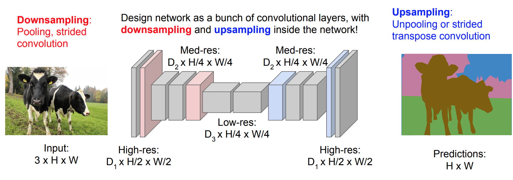
- We make use of convolutional networks by themselves, trained end-to-end, pixels-to-pixels.
-
- Structure:
- Input: Image vector
- Output: A Tensor \((C \times H \times W)\), where \(C\) is the number of classes.
- Structure:
- The key observation is that one can view Fully Connected Layers as Convolutions over the entire image.
Thus, the structure of the ConvNet is just a stacked number of convolutional layers that preserve the size of the image.- Issue with the Architecture:
The proposed approach of preserving the size of the input image leads to an exploding number of hyperparamters.
This makes training the network very tedious and it almost never converges. - Solution:
We allow the network to perform an encoding of the image by
first Downsampling the image,
then, Upsampling the image back, inside the network.
The Upsampling is not done via bicubic interpolation, instead, we use Deconvolutional layers (Unpooling) for learning the upsampling.
However, (even learnable)upsampling produces coarse segmentation maps because of loss of information during pooling. Therefore, shortcut/skip connections are introduced from higher resolution feature maps.
- Issue with the Architecture:
- Long et. al (2014)
Methods, Approaches and Algorithms in Training DL Models
-
- Upsampling:
- Also, known as “Unpooling”.
-
- Nearest Neighbor: fill each region with the corresponding pixel value in the original image.
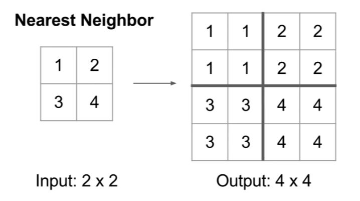
- Nearest Neighbor: fill each region with the corresponding pixel value in the original image.
-
- Bed of Nails: put each corresponding pixel value in the original image into the upper-left corner in each new sub-region, and fill the rest with zeros.
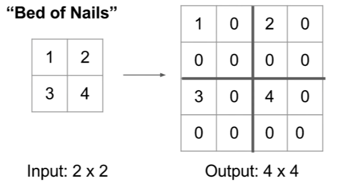
- Bed of Nails: put each corresponding pixel value in the original image into the upper-left corner in each new sub-region, and fill the rest with zeros.
-
- Max-Unpooling: The same idea as Bed of Nails, however, we re-place the pixel values from the original image into their original values that they were extracted from in the Max-Pooling step.

- Max-Unpooling: The same idea as Bed of Nails, however, we re-place the pixel values from the original image into their original values that they were extracted from in the Max-Pooling step.
-
- Learnable Upsampling: Deconvolutional Layers (Transpose Convolution):
-
- Transpose Convolution: is a convolution performed on a an input of a small size, each element in the input acts a scalar that gets multiplied by the filter, and then gets placed on a, larger, output matrix, where the regions of overlap get summed.
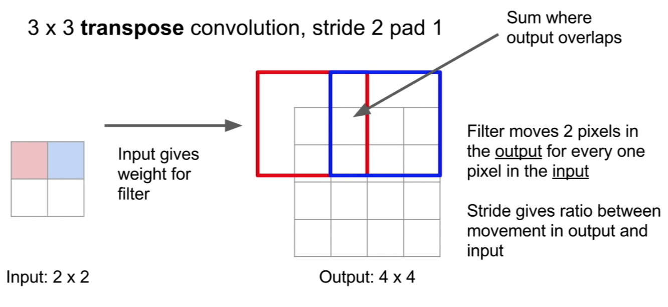
- Transpose Convolution: is a convolution performed on a an input of a small size, each element in the input acts a scalar that gets multiplied by the filter, and then gets placed on a, larger, output matrix, where the regions of overlap get summed.
- Also known as:
- Deconvolution
- UpConvolution
- Fractionally Strided Convolution
Reason: if you think of the stride as the ratio in step between the input and the output; this is equivalent to a stride one-half convolution, because of the ratio of 1-to-2 between the input and the output.
- Backward Strided Convolution
Reason: The forward pass of a Transpose Convolution is the same mathematical operation as the backward pass of a normal convolution.
-
- 1-D Example:
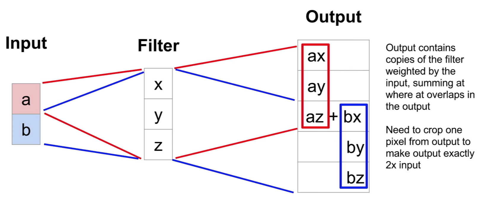
- 1-D Example:
-
- Convolution as Tensor Multiplication: All Convolutions (with stride and padding) can be framed as a Tensor Product by placing the filters intelligently in a tensor.
The name Transpose Convolution comes from the fact that the Deconvolution operation, viewed as a Tensor Product, is just the Transpose of the Convolution operation.- 1-D Example:
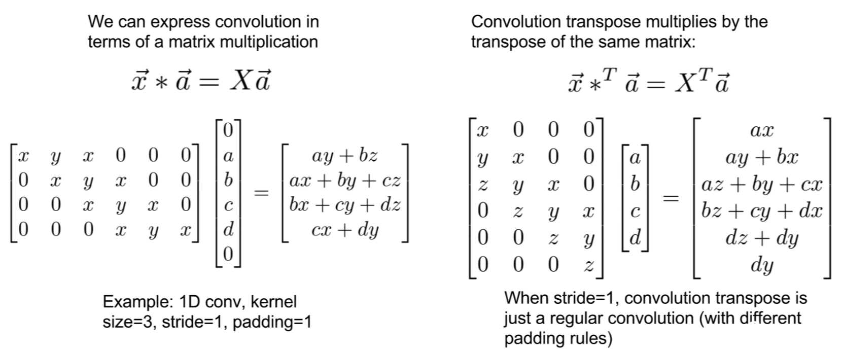
- In-fact, the name Deconvolution is a mis-nomer exactly because of this interpretation:
The Transpose matrix of the Convolution operation is a convolution iff the stride is equal to 1.
If the stride>1, then the transpose matrix no longer represents a convolution.
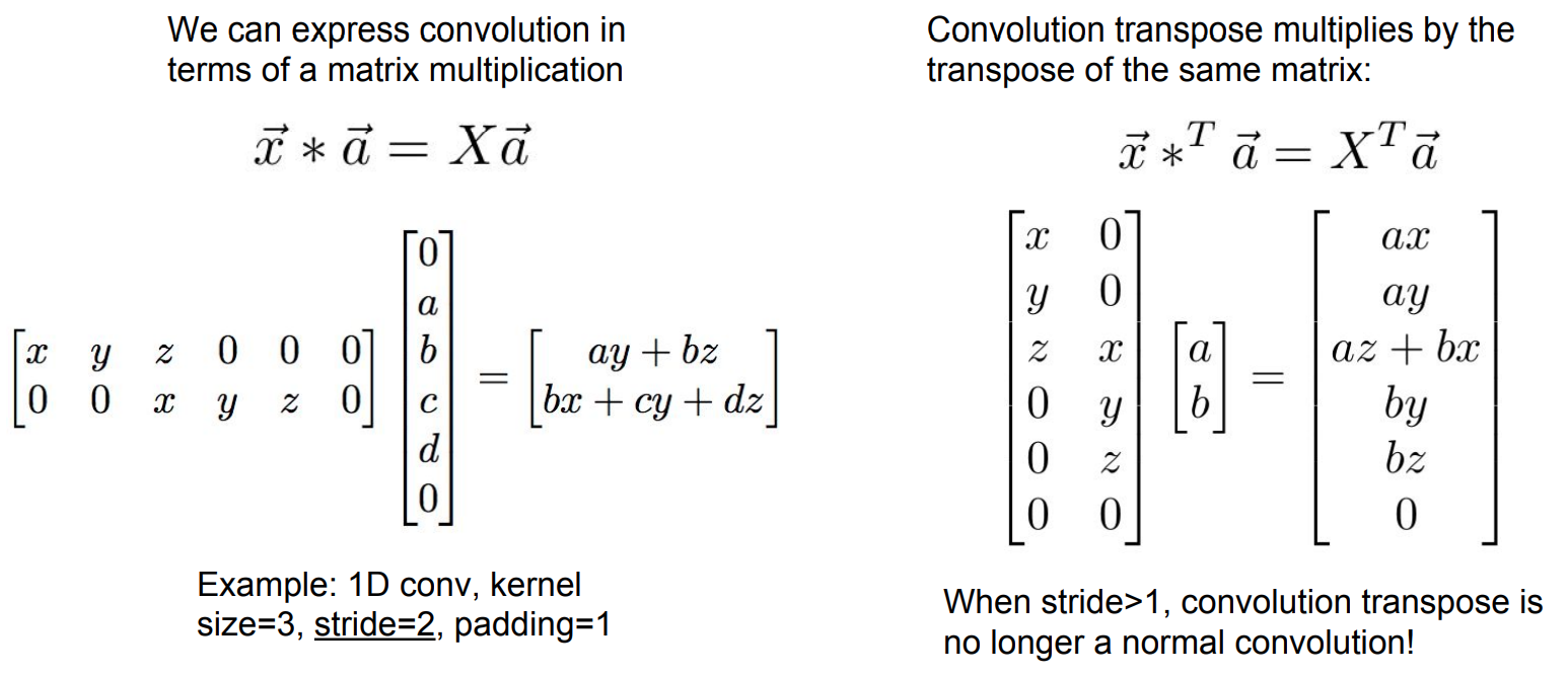
- 1-D Example:
- Convolution as Tensor Multiplication: All Convolutions (with stride and padding) can be framed as a Tensor Product by placing the filters intelligently in a tensor.
-
- Issues with Transpose Convolution:
- Since we sum the values that overlap in the region of the upsampled image, the magnitudes in the output will vary depending on the number of receptive fields in the output.
This leads to some checkerboard artifacts.
- Since we sum the values that overlap in the region of the upsampled image, the magnitudes in the output will vary depending on the number of receptive fields in the output.
- Solution:
- Avoid (3x3) stride two deconvolutions.
- Use (4x4) stride two, or (2x2) stride two deconvolutions.
- Issues with Transpose Convolution: