Ahmad Badary

Information Theory

A Short Introduction to Entropy, Cross-Entropy and KL-Divergence
Deep Learning Information Theory (Cross-Entropy and MLE)
Further Info (Lecture)
Visual Information Theory (Chris Olahs’ Blog) Deep Learning and Information Theory (Blog)
Information Theory | Statistics for Deep Learning (Blog)

Information Theory

Information Theory:
Information theory is a branch of applied mathematics that revolves around quantifying how much information is present in a signal.
In the context of machine learning, we can also apply information theory to continuous variables where some of these message length interpretations do not apply, instead, we mostly use a few key ideas from information theory to characterize probability distributions or to quantify similarity between probability distributions.
Motivation and Intuition:
The basic intuition behind information theory is that learning that an unlikely event has occurred is more informative than learning that a likely event has occurred. A message saying “the sun rose this morning” is so uninformative as to be unnecessary to send, but a message saying “there was a solar eclipse this morning” is very informative.
Thus, information theory quantifies information in a way that formalizes this intuition:
- Likely events should have low information content - in the extreme case, guaranteed events have no information at all
- Less likely events should have higher information content
- Independent events should have additive information. For example, finding out that a tossed coin has come up as heads twice should convey twice as much information as finding out that a tossed coin has come up as heads once.
Measuring Information:
In Shannons Theory, to transmit $1$ bit of information means to divide the recipients Uncertainty by a factor of $2$.

Thus, the amount of information transmitted is the logarithm (base $2$) of the uncertainty reduction factor.

The uncertainty reduction factor is just the inverse of the probability of the event being communicated.

Thus, the amount of information in an event $\mathbf{x} = x$, called the Self-Information is:

$$I(x) = \log (1/p(x)) = -\log(p(x))$$

Shannons Entropy:
It is the expected amount of information of an uncertain/stochastic source. It acts as a measure of the amount of uncertainty of the events.
Equivalently, the amount of information that you get from one sample drawn from a given probability distribution $p$.
Self-Information:
The Self-Information or surprisal is a synonym for the surprise when a random variable is sampled.
The Self-Information of an event $\mathrm{x} = x$:
$$I(x) = - \log P(x)$$

Self-information deals only with a single outcome.
Shannon Entropy:
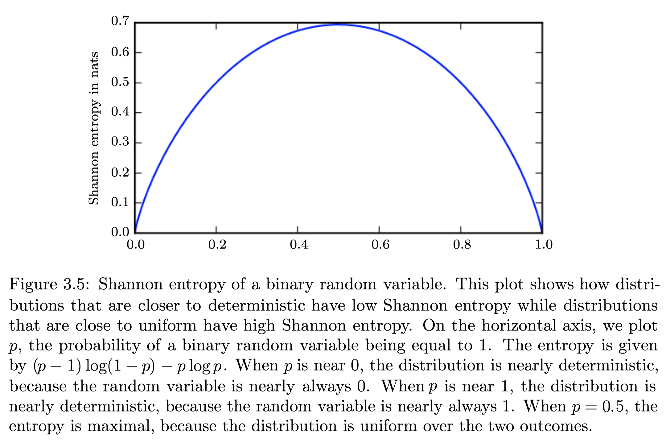
To quantify the amount of uncertainty in an entire probability distribution, we use Shannon Entropy.
Shannon Entropy is defined as the average amount of information produced by a stochastic source of data.
$$H(x) = {\displaystyle \operatorname {E}_{x \sim P} [I(x)]} = - {\displaystyle \operatorname {E}_{x \sim P} [\log P(X)] = -\sum_{i=1}^{n} p\left(x_{i}\right) \log p\left(x_{i}\right)}$$

Differential Entropy is Shannons entropy of a continuous random variable $x$.
Distributions and Entropy:
Distributions that are nearly deterministic (where the outcome is nearly certain) have low entropy; distributions that are closer to uniform have high entropy.
Relative Entropy | KL-Divergence:
The Kullback–Leibler divergence (Relative Entropy) is a measure of how one probability distribution diverges from a second, expected probability distribution.
Mathematically:
$${\displaystyle D_{\text{KL}}(P\parallel Q)=\operatorname{E}_{x \sim P} \left[\log \dfrac{P(x)}{Q(x)}\right]=\operatorname{E}_{x \sim P} \left[\log P(x) - \log Q(x)\right]}$$
- Discrete:
$${\displaystyle D_{\text{KL}}(P\parallel Q)=\sum_{i}P(i)\log \left({\frac {P(i)}{Q(i)}}\right)}$$
- Continuous:
$${\displaystyle D_{\text{KL}}(P\parallel Q)=\int_{-\infty }^{\infty }p(x)\log \left({\frac {p(x)}{q(x)}}\right)\,dx,}$$

Interpretation:
- Discrete variables:
  it is the extra amount of information needed to send a message containing symbols drawn from probability distribution $P$, when we use a code that was designed to minimize the length of messages drawn from probability distribution $Q$.
- Continuous variables:
Properties:
- Non-Negativity:
  ${\displaystyle D_{\mathrm {KL} }(P\|Q) \geq 0}$
- ${\displaystyle D_{\mathrm {KL} }(P\|Q) = 0 \iff}$ $P$ and $Q$ are:
  - Discrete Variables:
    the same distribution
  - Continuous Variables:
    equal “almost everywhere”
- Additivity of Independent Distributions:
  ${\displaystyle D_{\text{KL}}(P\parallel Q)=D_{\text{KL}}(P_{1}\parallel Q_{1})+D_{\text{KL}}(P_{2}\parallel Q_{2}).}$
- ${\displaystyle D_{\mathrm {KL} }(P\|Q) \neq D_{\mathrm {KL} }(Q\|P)}$
  
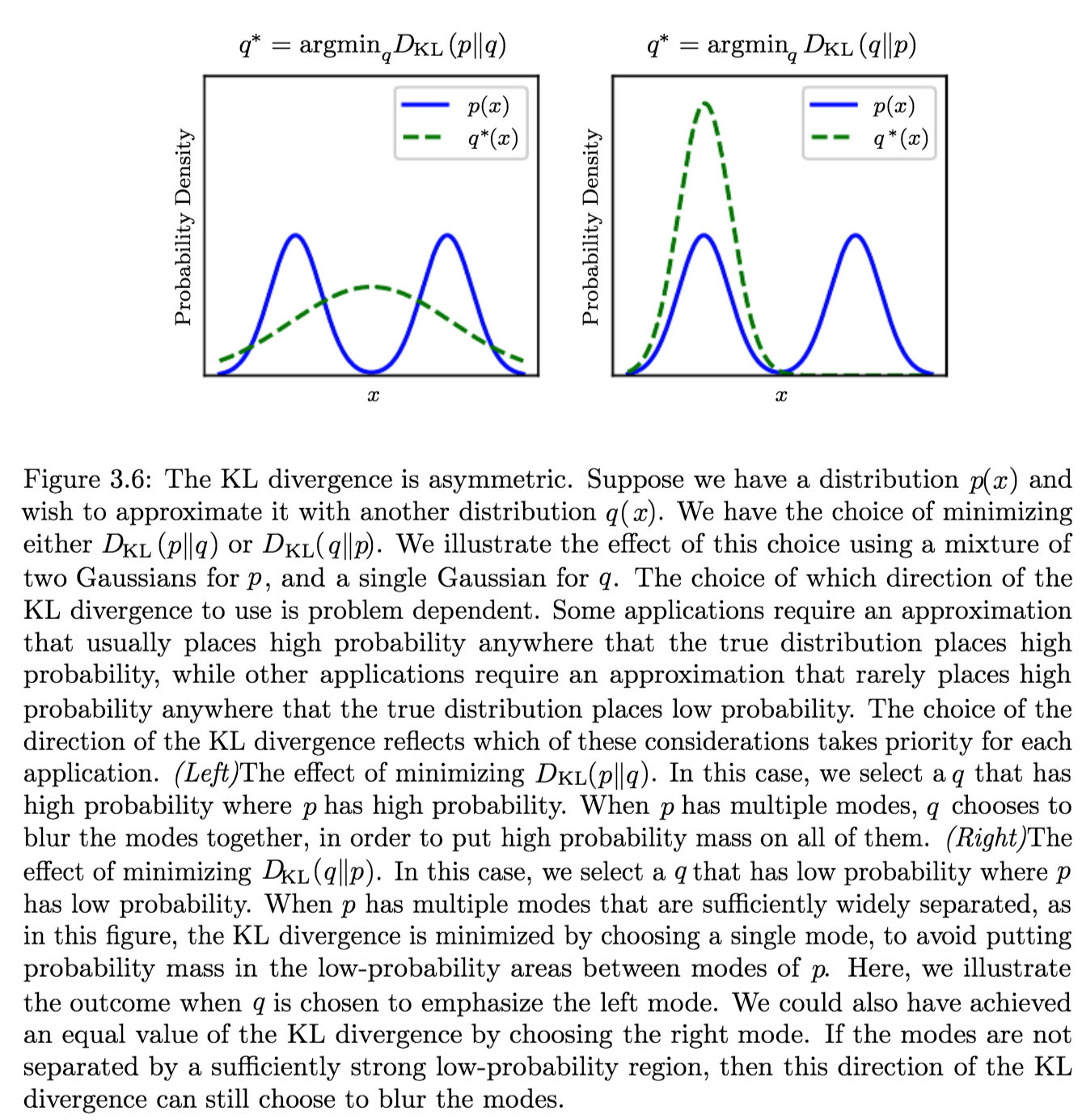
  This asymmetry means that there are important consequences to the choice of the ordering
- Convexity in the pair of PMFs $(p, q)$ (i.e. ${\displaystyle (p_{1},q_{1})}$ and ${\displaystyle (p_{2},q_{2})}$ are two pairs of PMFs):
  ${\displaystyle D_{\text{KL}}(\lambda p_{1}+(1-\lambda )p_{2}\parallel \lambda q_{1}+(1-\lambda )q_{2})\leq \lambda D_{\text{KL}}(p_{1}\parallel q_{1})+(1-\lambda )D_{\text{KL}}(p_{2}\parallel q_{2}){\text{ for }}0\leq \lambda \leq 1.}$
KL-Div as a Distance:
Because the KL divergence is non-negative and measures the difference between two distributions, it is often conceptualized as measuring some sort of distance between these distributions.
However, it is not a true distance measure because it is not symmetric.

KL-div is, however, a Quasi-Metric, since it satisfies all the properties of a distance-metric except symmetry

Applications
Characterizing:
- Relative (Shannon) entropy in information systems
- Randomness in continuous time-series
- It is a measure of Information Gain; used when comparing statistical models of inference
Example Application and Direction of Minimization
Suppose we have a distribution $p(x)$ and we wish to approximate it with another distribution $q(x)$.
We have a choice of minimizing either:
1. ${\displaystyle D_{\text{KL}}(p\|q)} \implies q^\ast = \operatorname {arg\,min}_q {\displaystyle D_{\text{KL}}(p\|q)}$
  Produces an approximation that usually places high probability anywhere that the true distribution places high probability.
2. ${\displaystyle D_{\text{KL}}(q\|p)} \implies q^\ast \operatorname {arg\,min}_q {\displaystyle D_{\text{KL}}(q\|p)}$
  Produces an approximation that rarely places high probability anywhere that the true distribution places low probability.
  
  which are different due to the asymmetry of the KL-divergence
Cross Entropy:
The Cross Entropy between two probability distributions ${\displaystyle p}$ and ${\displaystyle q}$ over the same underlying set of events measures the average number of bits needed to identify an event drawn from the set, if a coding scheme is used that is optimized for an “unnatural” probability distribution ${\displaystyle q}$, rather than the “true” distribution ${\displaystyle p}$.
$$H(p,q) = \operatorname{E}_{p}[-\log q]= H(p) + D_{\mathrm{KL}}(p\|q) =-\sum_{x }p(x)\,\log q(x)$$

It is similar to KL-Div but with an additional quantity - the entropy of $p$.

Minimizing the cross-entropy with respect to $Q$ is equivalent to minimizing the KL divergence, because $Q$ does not participate in the omitted term.

We treat $0 \log (0)$ as $\lim_{x \to 0} x \log (x) = 0$.
Mutual Information:
The Mutual Information (MI) of two random variables is a measure of the mutual dependence between the two variables.
More specifically, it quantifies the “amount of information” (in bits) obtained about one random variable through observing the other random variable.

It can be seen as a way of measuring the reduction in uncertainty (information content) of measuring a part of the system after observing the outcome of another parts of the system; given two R.Vs, knowing the value of one of the R.Vs in the system gives a corresponding reduction in (the uncertainty (information content) of) measuring the other one.

As KL-Divergence:
Let $(X, Y)$ be a pair of random variables with values over the space $\mathcal{X} \times \mathcal{Y}$ . If their joint distribution is $P_{(X, Y)}$ and the marginal distributions are $P_{X}$ and $P_{Y},$ the mutual information is defined as:

$$I(X ; Y)=D_{\mathrm{KL}}\left(P_{(X, Y)} \| P_{X} \otimes P_{Y}\right)$$

In terms of PMFs for discrete distributions:
The mutual information of two jointly discrete random variables $X$ and $Y$ is calculated as a double sum:

$$\mathrm{I}(X ; Y)=\sum_{y \in \mathcal{Y}} \sum_{x \in \mathcal{X}} p_{(X, Y)}(x, y) \log \left(\frac{p_{(X, Y)}(x, y)}{p_{X}(x) p_{Y}(y)}\right)$$

where ${\displaystyle p_{(X,Y)}}$ is the joint probability mass function of ${\displaystyle X}$ X and ${\displaystyle Y}$, and ${\displaystyle p_{X}}$ and ${\displaystyle p_{Y}}$ are the marginal probability mass functions of ${\displaystyle X}$ and ${\displaystyle Y}$ respectively.

In terms of PDFs for continuous distributions:
In the case of jointly continuous random variables, the double sum is replaced by a double integral:

$$\mathrm{I}(X ; Y)=\int_{\mathcal{Y}} \int_{\mathcal{X}} p_{(X, Y)}(x, y) \log \left(\frac{p_{(X, Y)}(x, y)}{p_{X}(x) p_{Y}(y)}\right) d x d y$$

where $p_{(X, Y)}$ is now the joint probability density function of $X$ and $Y$ and $p_{X}$ and $p_{Y}$ are the marginal probability density functions of $X$ and $Y$ respectively.

Intuitive Definitions:
- Measures the information that $X$ and $Y$ share:
  It measures how much knowing one of these variables reduces uncertainty about the other.
  - $X, Y$ Independent $\implies I(X; Y) = 0$: their MI is zero
  - $X$ deterministic function of $Y$ and vice versa $\implies I(X; Y) = H(X) = H(Y)$ their MI is equal to entropy of each variable
- It’s a Measure of the inherent dependence expressed in the joint distribution of $X$ and $Y$ relative to the joint distribution of $X$ and $Y$ under the assumption of independence.
  i.e. The price for encoding ${\displaystyle (X,Y)}$ as a pair of independent random variables, when in reality they are not.
Properties:
- The KL-divergence shows that $I(X; Y)$ is equal to zero precisely when the joint distribution conicides with the product of the marginals i.e. when $X$ and $Y$ are independent.
- The MI is non-negative: $I(X; Y) \geq 0$
  - It is a measure of the price for encoding ${\displaystyle (X,Y)}$ as a pair of independent random variables, when in reality they are not.
- It is symmetric: $I(X; Y) = I(Y; X)$
- Related to conditional and joint entropies:
  $${\displaystyle {\begin{aligned}\operatorname {I} (X;Y)&{}\equiv \mathrm {H} (X)-\mathrm {H} (X|Y)\\&{}\equiv \mathrm {H} (Y)-\mathrm {H} (Y|X)\\&{}\equiv \mathrm {H} (X)+\mathrm {H} (Y)-\mathrm {H} (X,Y)\\&{}\equiv \mathrm {H} (X,Y)-\mathrm {H} (X|Y)-\mathrm {H} (Y|X)\end{aligned}}}$$
  
  where $\mathrm{H}(X)$ and $\mathrm{H}(Y)$ are the marginal entropies, $\mathrm{H}(X | Y)$ and $\mathrm{H}(Y | X)$ are the conditional entopries, and $\mathrm{H}(X, Y)$ is the joint entropy of $X$ and $Y$.
  - Note the analogy to the union, difference, and intersection of two sets:
- Related to KL-div of conditional distribution:
  $$\mathrm{I}(X ; Y)=\mathbb{E}_{Y}\left[D_{\mathrm{KL}}\left(p_{X | Y} \| p_{X}\right)\right]$$
- MI (tutorial #1)
- MI (tutorial #2)
Applications:
- In search engine technology, mutual information between phrases and contexts is used as a feature for k-means clustering to discover semantic clusters (concepts)
- Discriminative training procedures for hidden Markov models have been proposed based on the maximum mutual information (MMI) criterion.
- Mutual information has been used as a criterion for feature selection and feature transformations in machine learning. It can be used to characterize both the relevance and redundancy of variables, such as the minimum redundancy feature selection.
- Mutual information is used in determining the similarity of two different clusterings of a dataset. As such, it provides some advantages over the traditional Rand index.
- Mutual information of words is often used as a significance function for the computation of collocations in corpus linguistics.
- Detection of phase synchronization in time series analysis
- The mutual information is used to learn the structure of Bayesian networks/dynamic Bayesian networks, which is thought to explain the causal relationship between random variables
- Popular cost function in decision tree learning.
- In the infomax method for neural-net and other machine learning, including the infomax-based Independent component analysis algorithm
Independence assumptions and low-rank matrix approximation (alternative definition):

As a Metric (relation to Jaccard distance):
Pointwise Mutual Information (PMI):
The PMI of a pair of outcomes $x$ and $y$ belonging to discrete random variables $X$ and $Y$ quantifies the discrepancy between the probability of their coincidence given their joint distribution and their individual distributions, assuming independence. Mathematically:
$$\operatorname{pmi}(x ; y) \equiv \log \frac{p(x, y)}{p(x) p(y)}=\log \frac{p(x | y)}{p(x)}=\log \frac{p(y | x)}{p(y)}$$

In contrast to mutual information (MI) which builds upon PMI, it refers to single events, whereas MI refers to the average of all possible events.
The mutual information (MI) of the random variables $X$ and $Y$ is the expected value of the PMI (over all possible outcomes).

Conditional Entropy: $H(X \mid Y)=H(X)-I(X, Y)$
Independence: $I(X, Y)=0$
Independence Relations: $H(X \mid Y)=H(X)$

Information Theory

Table of Contents

Information Theory

More