Table of Contents
Lecture on Statistical Learning Theory from Risk perspective & Bayes Decision Rule
Learning Theory Andrew NG (CS229 Stanford)
Empirical Risk Minimization (Cornell)
Fundamental Problem of Machine Learning: It is Ill-Posed:
Learning appears impossible: Learning a truly “unknown” function is impossible.

- Solution: Work with a Restricted Hypothesis Space:
Either by applying prior knowledge or by guessing, we choose a space of hypotheses \(H\) that is smaller than the space of all possible functions:-
simple conjunctive rules, linear functions, multivariate Gaussian joint probability distributions, etc.
-
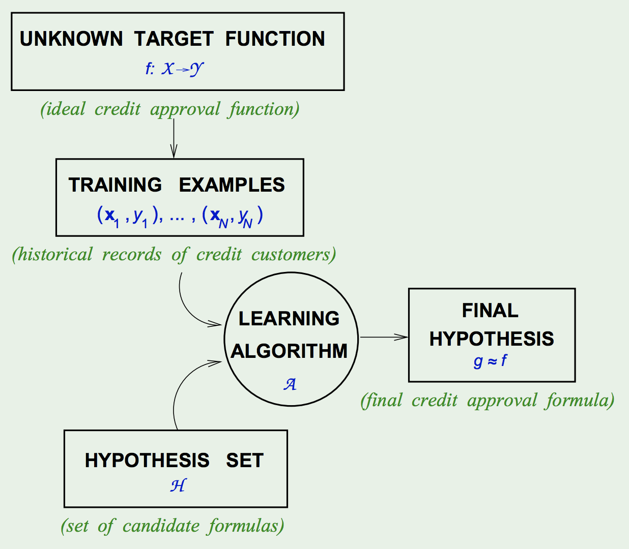
Lets say you have an unknown target function \(f: X \rightarrow Y\) that you are trying to capture by learning. In order to capture the target function you have to come up with (guess) some hypotheses \(h_{1}, \ldots, h_{n}\) where \(h \in H\), and then search through these hypotheses to select the best one that approximates the target function.
-
Two Views of Learning and their corresponding Strategies:
- Learning is the removal of our remaining uncertainty
– Suppose we knew that the unknown function was an m-of-n boolean function. Then we could use the training examples to deduce which function it is.
– Our prior “knowledge” might be wrong- Strategy: Develop Languages for Expressing Prior Knowledge
Rule grammars, stochastic models, Bayesian networks
- Strategy: Develop Languages for Expressing Prior Knowledge
- Learning requires guessing a good, small hypothesis class.
– We can start with a very small class and enlarge it until it contains an hypothesis that fits the data.
– Our guess of the hypothesis class could be wrong: The smaller the class, the more likely we are wrong.- Strategy: Develop Flexible Hypothesis Spaces
Nested collections of hypotheses: decision trees, neural networks, cases, SVMs
- Strategy: Develop Flexible Hypothesis Spaces
Key Issues in Machine Learning:
- What are good hypothesis spaces?
- which spaces have been useful in practical applications?
- What algorithms can work with these spaces?
- Are there general design principles for learning algorithms?
- How can we optimize accuracy on future data points?
- This is related to the problem of “overfitting”
- How can we have confidence in the results? (the statistical question)
- How much training data is required to find an accurate hypotheses?
- Are some learning problems computational intractable? (the computational question)
- How can we formulate application problems as machine learning problems? (the engineering question)
A Framework for Hypothesis Spaces:
- Size: Does the hypothesis space have a fixed size or a variable size?
- Fixed-sized spaces are easier to understand, but variable-sized spaces are generally more useful.
- Variable-sized spaces introduce the problem of overfiting.
- Stochasticity: Is the hypothesis a classifier, a conditional distribution, or a joint distribution?
This affects how we evaluate hypotheses.- For a deterministic hypothesis, a training example is either consistent (correctly predicted) or inconsistent (incorrectly predicted).
- For a stochastic hypothesis, a training example is more likely or less likely.
- Parameterization: Is each hypothesis described by a set of symbolic (discrete) choices or is it described by a set of continuous parameters?
If both are required, we say the space has a mixed parameterization.- Discrete parameters must be found by combinatorial search methods
- Continuous parameters can be found by numerical search methods
-

Note: LTU == Linear Threshold Unit.
A Framework for Learning Algorithms:
The Learning Problem
- When to use ML:
When:- A pattern Exists
- We cannot pin the pattern down mathematically
- We have Data
We usually can do without the first two. But the third condition we CANNOT do without.
The Theory of Learning only depends on the data.“We have to have data. We are learning from data. So if someone knocks on my door with an interesting machine learning application, and they tell me how exciting it is, and how great the application would be, and how much money they would make, the first question I ask, ‘what data do you have?’. If you have data, we are in business. If you don’t, you are out of luck.” - Prof. Ng
- The ML Approach to Problem Solving:
Consider the Netflix problem: Predicting how a viewer will rate a movie.- Direct Approach:
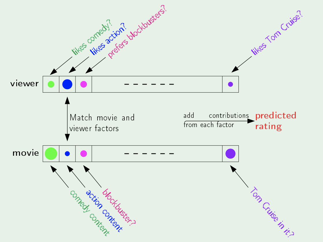
- Ask each user to give a rank/rate for the different “factors/features” (E.g. Action, Comedy, etc.)
- Watch each movie and assign a rank/rate for the same factors
- Match the factors and produce a rating
- ML Approach:
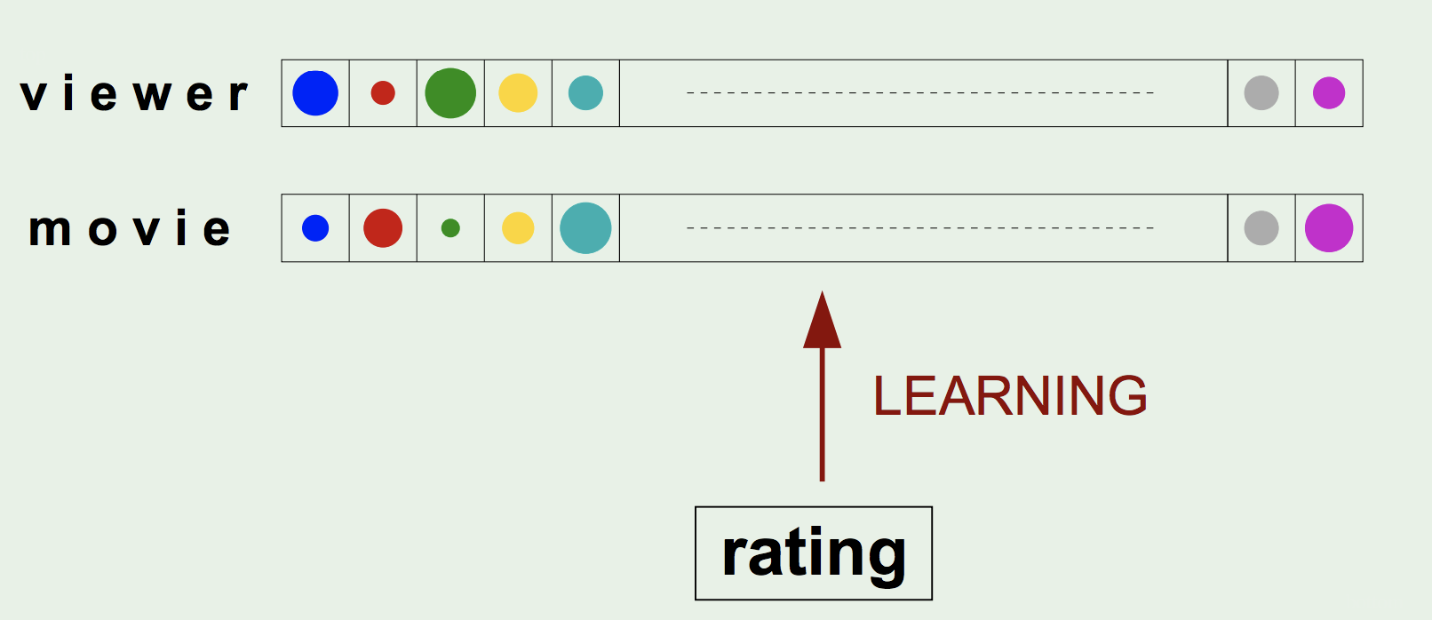
Essentially it is a Reversed approach- Start with the Ratings (dataset) that the users assigned to each movie
- Then deduce the “factors/features” that are consistent with those Ratings
Note: we usually start with random initial numbers for the factors
- Direct Approach:
- Components of Learning:
- Input: \(\vec{x}\)
- Output: \(y\)
- Data: \({(\vec{x}_ 1, y_ 1), (\vec{x}_ 2, y_ 2), ..., (\vec{x}_ N, y_ N)}\)
- Target Function: \(f : \mathcal{X} \rightarrow \mathcal{Y}\) (Unknown/Unobserved)
- Hypothesis: \(g : \mathcal{X} \rightarrow \mathcal{Y}\)
- Components of the Solution:
- The Learning Model:
- The Hypothesis Set: \(\mathcal{H}=\{h\}, g \in \mathcal{H}\)
E.g. Perceptron, SVM, FNNs, etc.
- The Learning Algorithm: picks \(g \approx f\) from a hypothesis set \(\mathcal{H}\)
E.g. Backprop, Quadratic Programming, etc.
- The Hypothesis Set: \(\mathcal{H}=\{h\}, g \in \mathcal{H}\)
Motivating the inclusion of a Hypothesis Set:
- No Downsides: There is no loss of generality by including a hypothesis set, since any restrictions on the elements of the set have no effect on what the learning algorithms
Basically, there is no downside because from a practical POV thats what you do; by choosing an initial approach, e.g. SVM, Linear Regression, Neural Network, etc., we are already dictating a hypothesis set. If we don’t choose one, then the hypothesis set has no restrictions and is the set of all possible hypothesis without loss of generalization. - Upside: The hypothesis set plays a pivotal role in the theory of learning, by dictating whether we can learn or not.
- The Learning Model:
-
The Basic Premise/Goal of Learning:
“Using a set of observations to uncover an underlying process”
Rephrased mathematically, the Goal of Learning is:
Use the Data to find a hypothesis \(g \in \mathcal{H}\), from the hypothesis set \(\mathcal{H}=\{h\}\), that approximates \(f\) well.
- Types of Learning:
- Supervised Learning: the task of learning a function that maps an input to an output based on example input-output pairs.
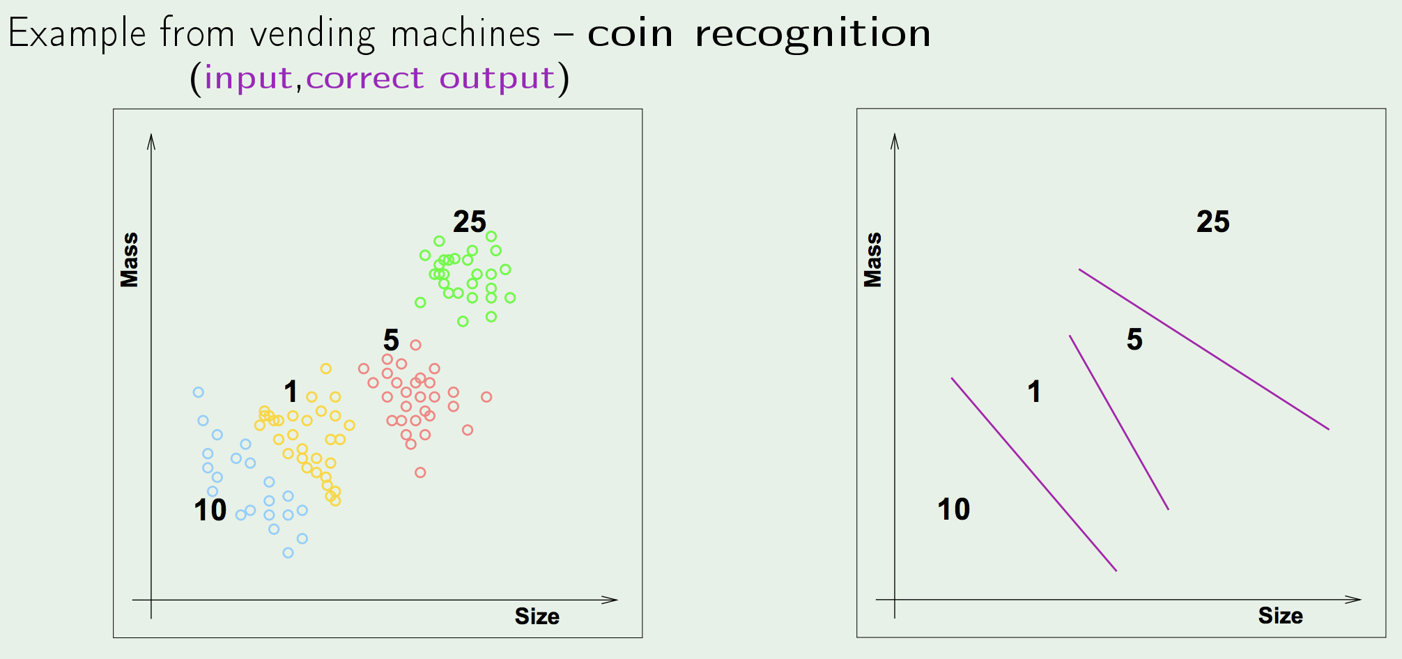
- Unsupervised Learning: the task of making inferences, by learning a better representation, from some datapoints that do not have any labels associated with them.
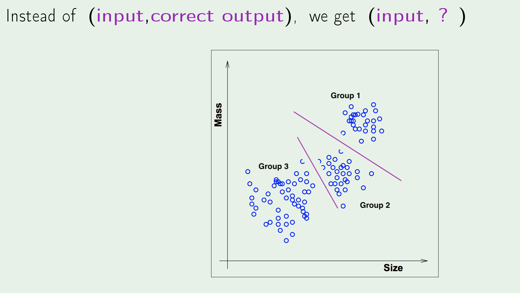
Unsupervised Learning is another name for Hebbian Learning
- Reinforcement Leaning: the task of learning how software agents ought to take actions in an environment so as to maximize some notion of cumulative reward.
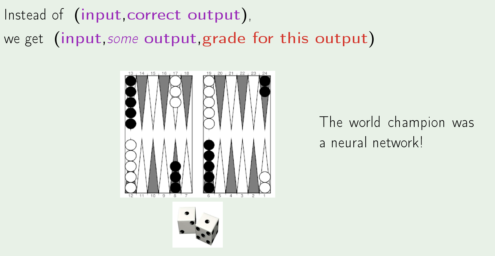
- Supervised Learning: the task of learning a function that maps an input to an output based on example input-output pairs.
- The Learning Diagram:
The Feasibility of Learning
The Goal of this Section is to answer the question: Can we make any statements/inferences outside of the sample data that we have?
-
The Problem of Learning:
Learning a truly Unknown function is Impossible, since outside of the observed values, the function could assume any value it wants. - The Bin Analogy - A Related Experiment::
-
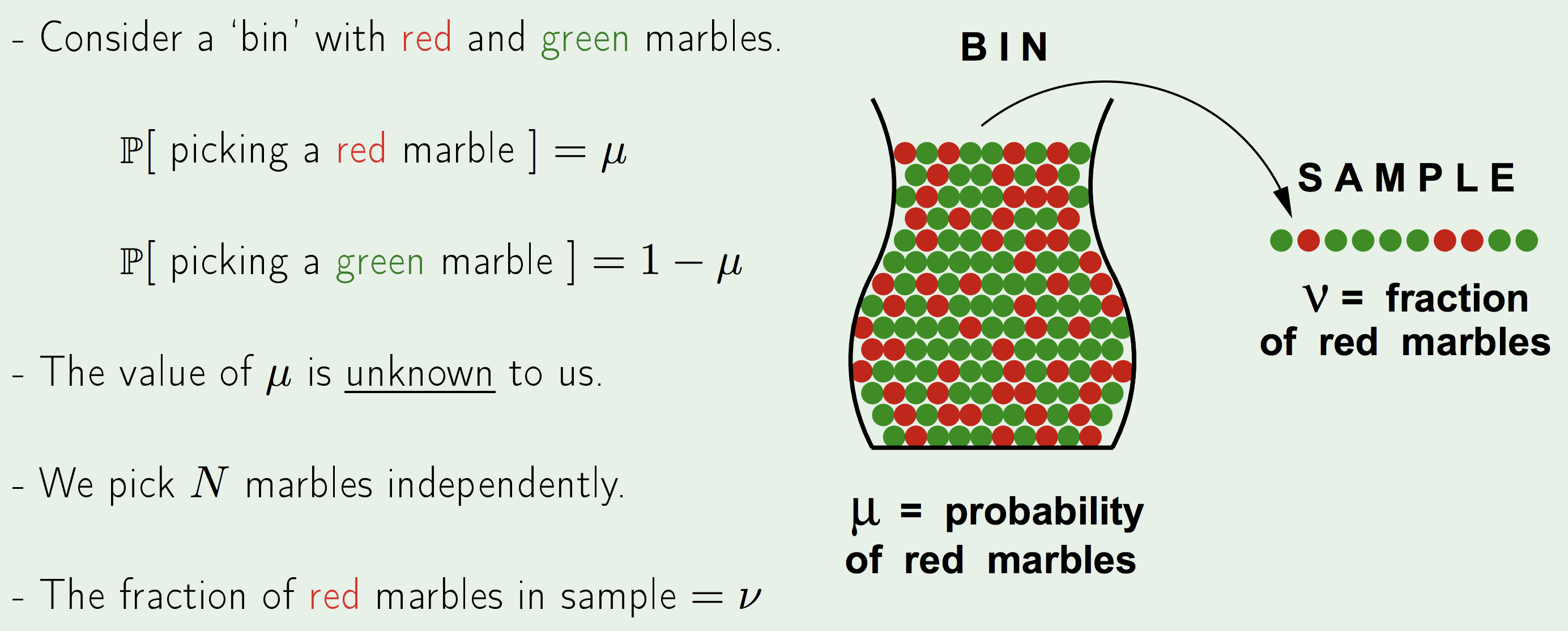
\(\mu\) is a constant that describes the actual/real probability of picking the red marble.
\(\nu\), however, is random and depends on the frequency of red marbles in the particular sample that you have collected.Does \(\nu\) approximate \(\mu\)?
- The short answer is NO:
The Sample an be mostly green while bin is mostly red. - The Long answer is YES:
The Sample frequency \(\nu\) is likely/probably close to bin frequency \(\mu\).Think of a presidential poll of 3000 people that can predict how the larger \(10^8\) mil. people will vote
The Main distinction between the two answers is in the difference between Possible VS Probable.
What does \(\nu\) say about \(\mu\)?
In a big sample (Large \(N\)), \(\nu\) is probably close to \(\mu\) (within \(\epsilon\)).
Formally, we the Hoeffding’s Inequality:$$\mathbb{P}[|\nu-\mu|>\epsilon] \leq 2 e^{-2 \epsilon^{2} N}$$
In other words, the probability that \(\nu\) does not approximate \(\mu\) well (they are not within an \(\epsilon\) of each other), is bounded by a negative exponential that dampens fast but depends directly on the tolerance \(\epsilon\).
This reduces to the statement that “\(\mu = \nu\)” is PAC (PAC: Probably, Approximately Correct).
Properties:
- It is valid for \(N\) and \(\epsilon\).
- The bound does not depend on the value of \(\mu\).
- There is a Trade-off between the number of samples \(N\) and the tolerance \(\epsilon\).
- Saying that \(\nu \approx \mu \implies \mu \approx \nu\), i.e. saying \(\nu\) is approximately the same as \(\mu\), implies that \(\mu\) is approximately the same as \(\nu\) (yes, tautology).
The logic here is subtle:- Logically, the inequality is making a statement on \(\nu\) (the random variable), it is saying that \(\nu\) tends to be close to \(\mu\) (the constant, real probability).
- However, since the inequality is symmetric, we are using the inequality to infer \(\mu\) from \(\nu\).
But that is not the cause and effect that actually takes place. \(\mu\), actually, affects \(\nu\).
Translating to the Learning Problem:
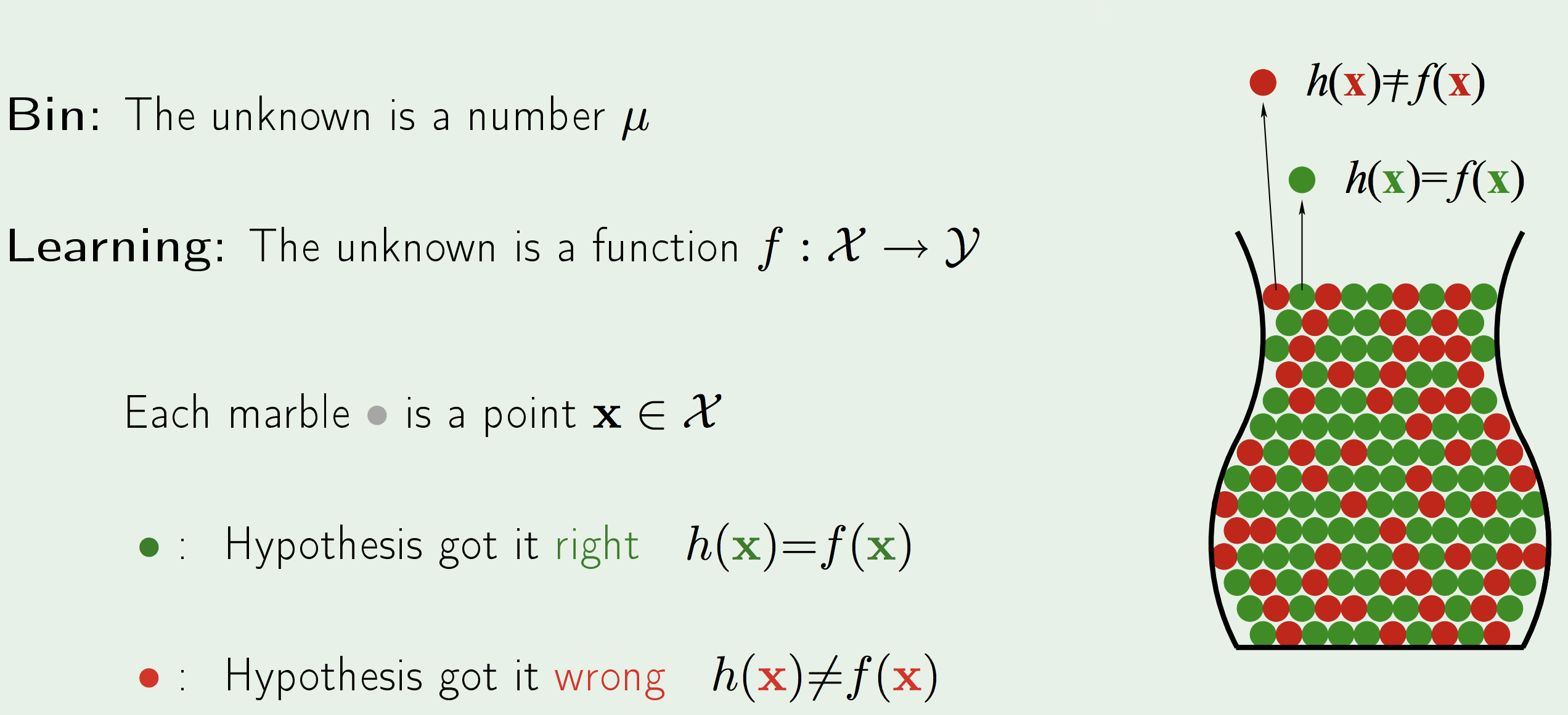
Notice how the meaning of the accordance between \(\mu\) and \(\nu\) is not accuracy of the model, but rather accuracy of the TEST.
Back to the Learning Diagram:
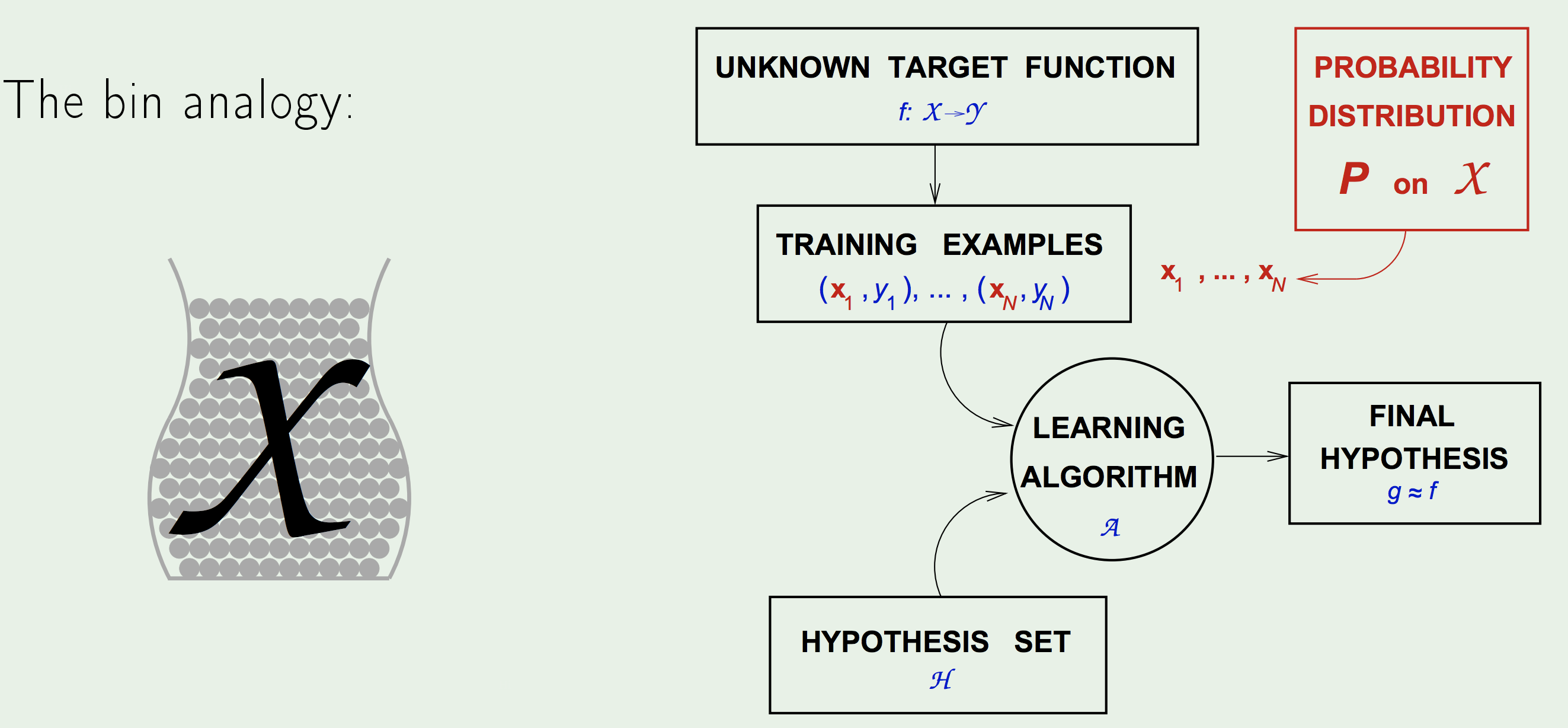
The marbles in the bin correspond to the input space (datapoints). This adds a NEW COMPONENT to the Learning problem - the probability of generating the input datapoints (up to this point we treated learning in an absolute sense based on some fixed datapoints).
To adjust the statement of the learning problem to accommodate the new component:
we add a probability distribution \(P\) over the input space \(\mathcal{X}\). This, however, doesn’t restrict the argument at all; we can invoke any probability on the space, and the machinery still holds. We, also, do not, even, need to know what \(P\) is (even though \(P\) affects \(\mu\)), since Hoeffding’s Inequality allows us to bound the LHS with no dependence on \(\mu\).
Thus, now we assume that the input datapoints \(\vec{x}_1, ..., \vec{x}_N\) are assumed to be generated by \(P\), independently.
So this is a very benign addition, that would give us high dividends - The Feasibility of Learning.However, this is not learning; it is Verification. Learning involves using an algorithm to search a space \(\mathcal{H}\) and try different functions \(h \in \mathcal{H}\). Here, we have already picked some specific function and are testing its performance on a sample, using maths to guarantee the accuracy of the test within some threshold we are willing to tolerate.
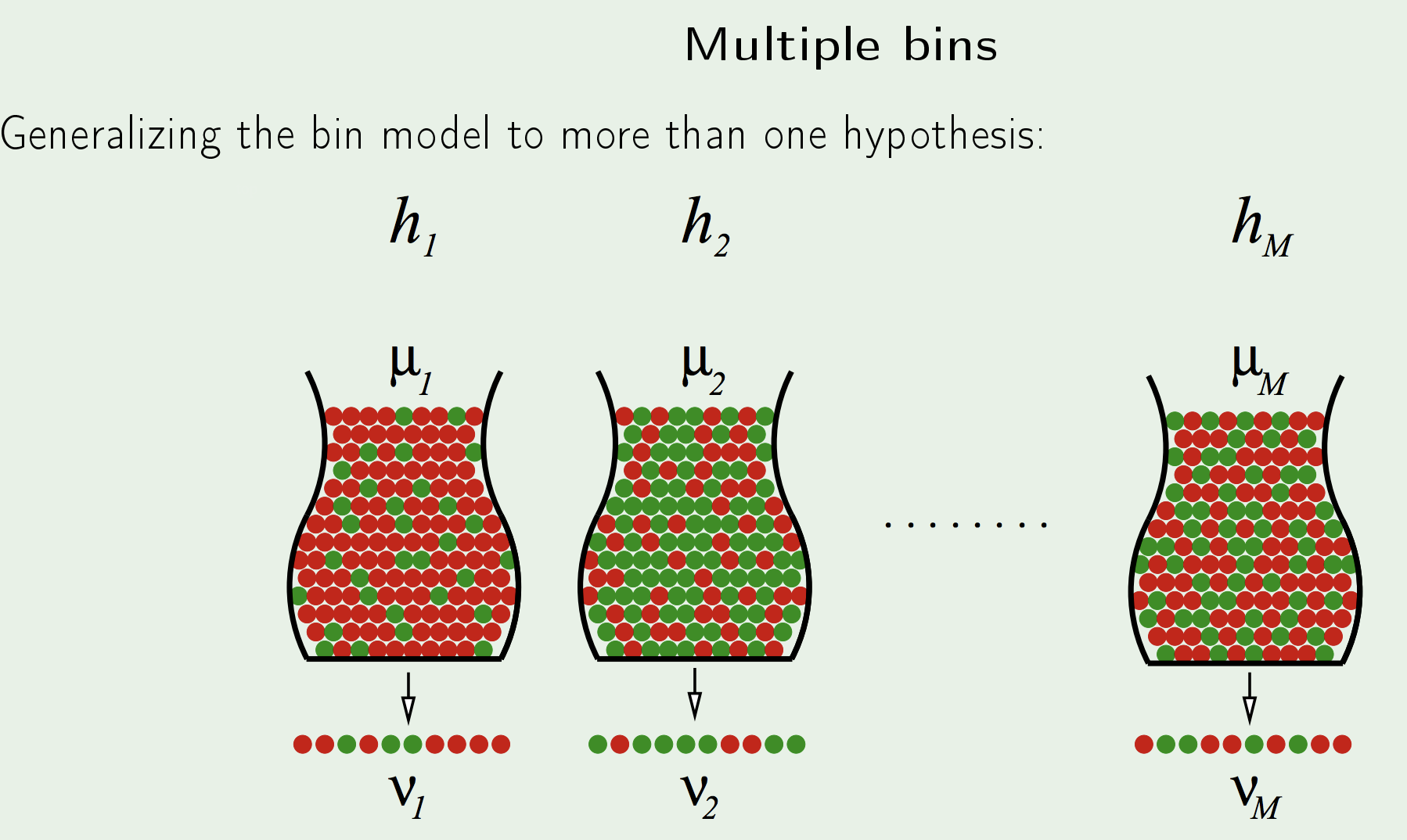
Extending Hoeffding’s Inequality to Multiple hypotheses \(h_i\):
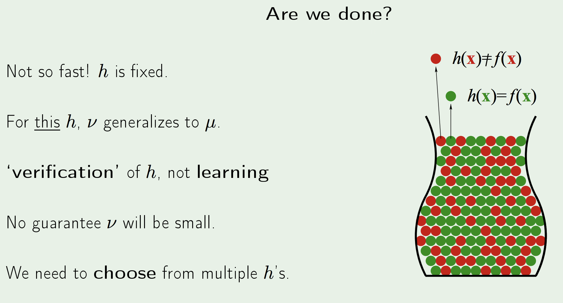
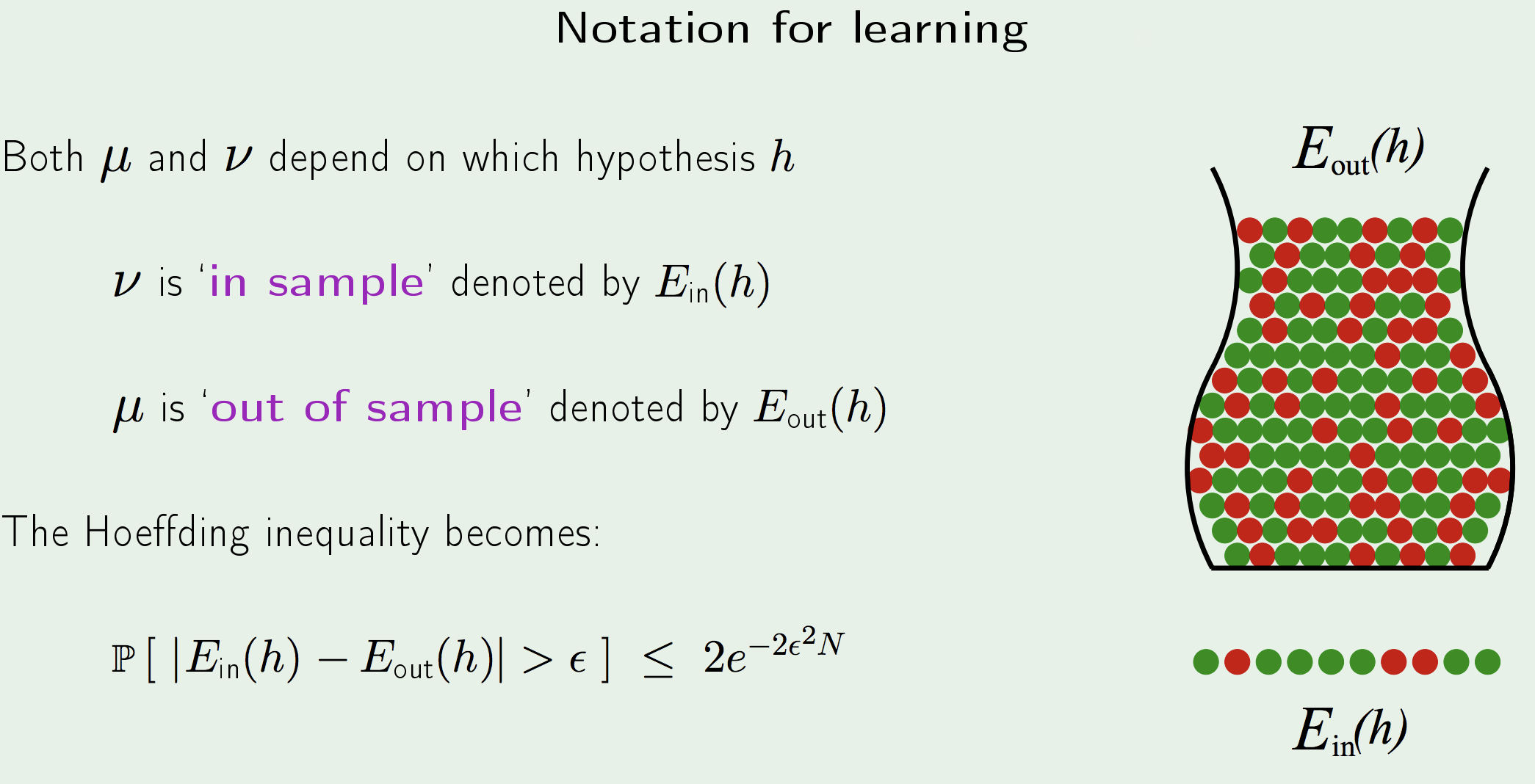
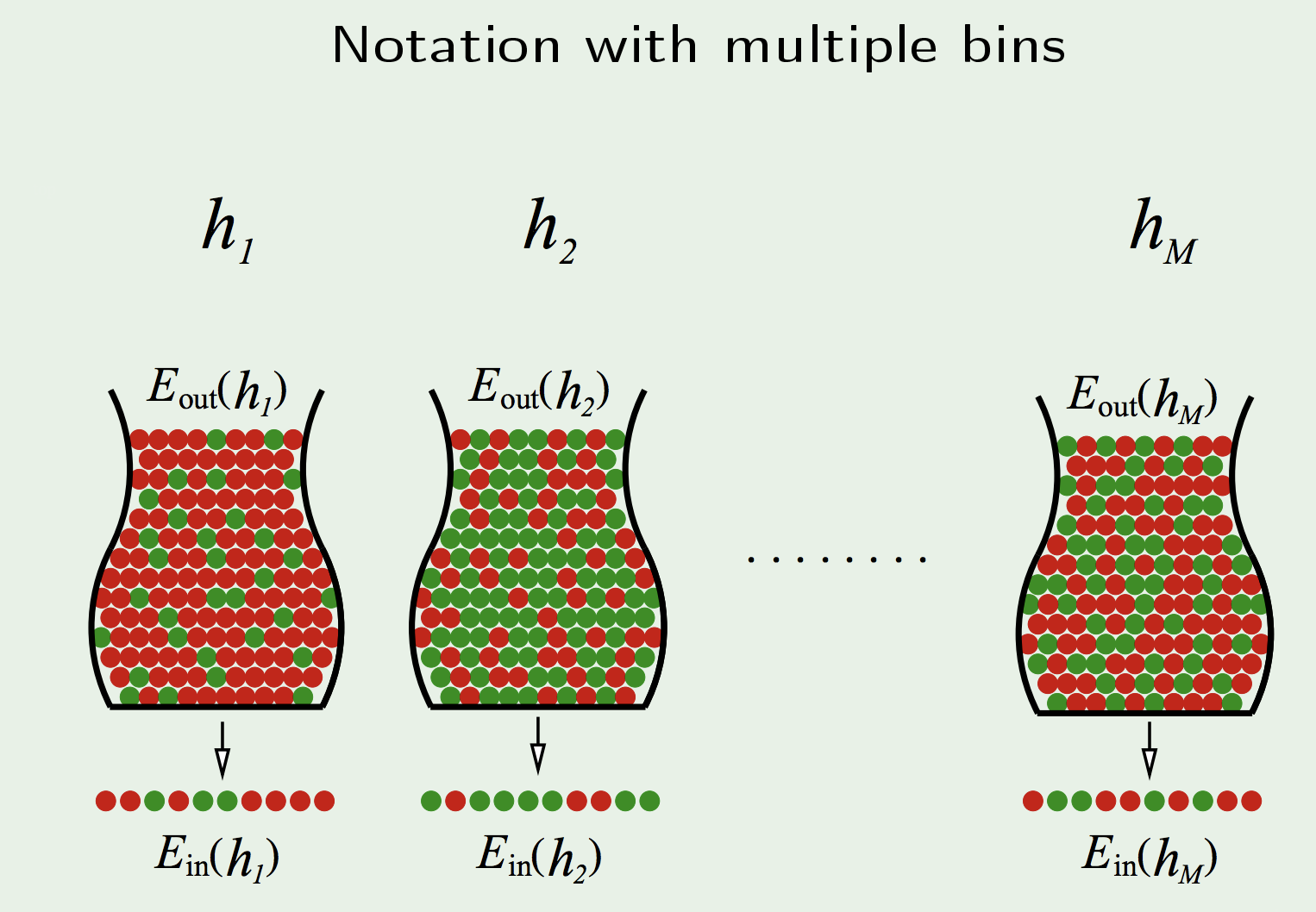
Putting the right notation:
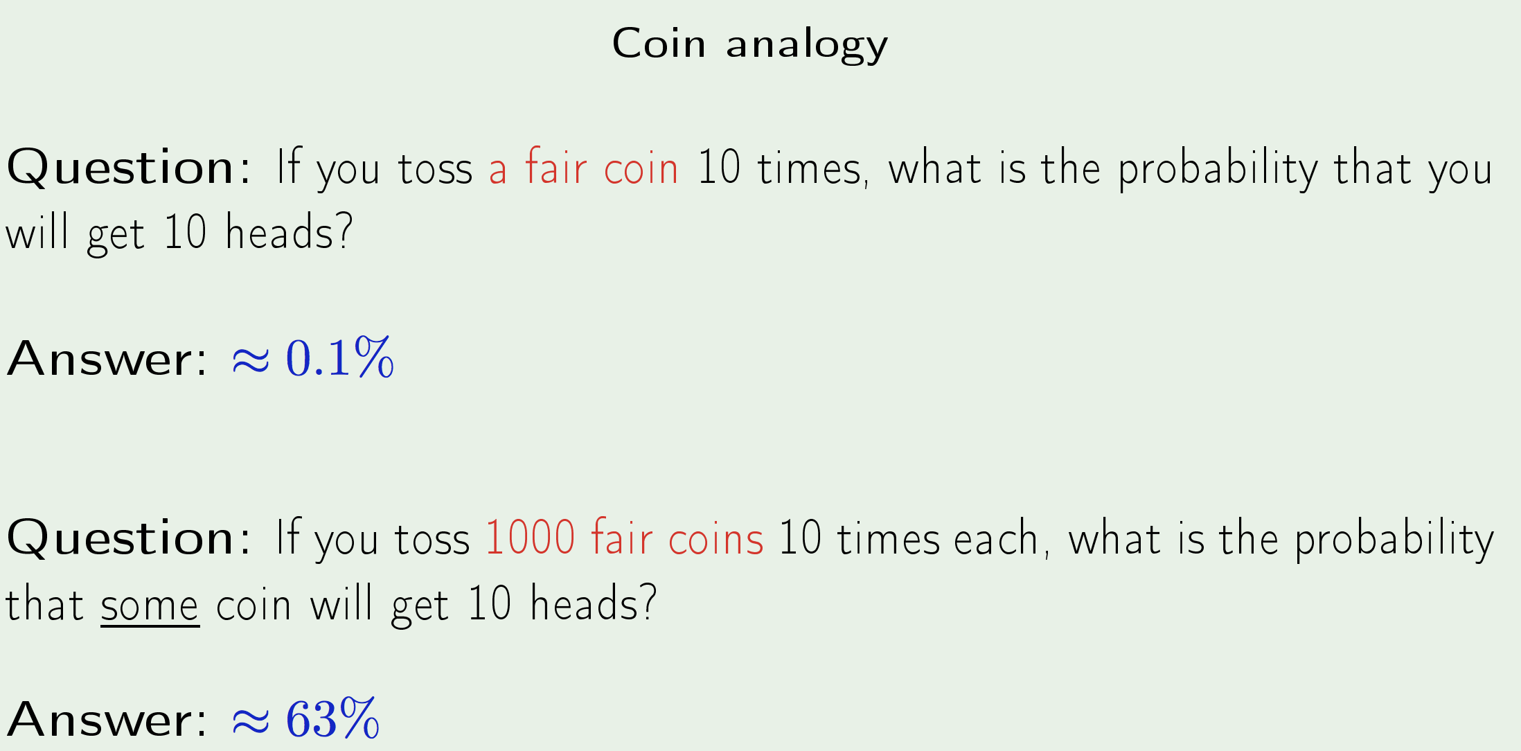
i.e. the 10 heads are not a good indication of the real probability
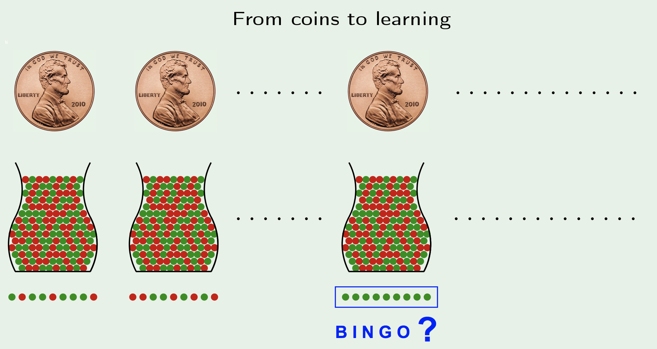
Equivalently, in learning, if the hypothesis set size is 1000, and there are 10 points we test against, the probability that one of those hypothesis performing well on the 10 points, but actually being a bad hypothesis is high, and increases with the hypothesis set size.Hoeffding’s inequality has a guarantee for one experiment, that gets terribly diluted as you increase the number of experiments.
Solution:
We follow the very same reasoning: we want to know the probability of at least one failing. This can be bounded by the union bound, which intuitively says that the maximum probability of at least an event occurring in N is when all the events are independent, in which case you just sum up the probabilities:$$\begin{aligned} \mathbb{P}\left[ | E_{\text {in }}(g)-E_{\text {out }}(g) |>\epsilon\right] \leq \mathbb{P}[ & | E_{\text {in }}\left(h_{1}\right)-E_{\text {out }}\left(h_{1}\right) |>\epsilon \\ & \text {or } | E_{\text {in }}\left(h_{2}\right)-E_{\text {out }}\left(h_{2}\right) |>\epsilon \\ & \cdots \\ & \text {or } | E_{\text {in }}\left(h_{M}\right)-E_{\text {out }}\left(h_{M}\right) |>\epsilon ] \\ \leq & \sum_{m=1}^{M} \mathbb{P}\left[ | E_{\text {in }}\left(h_{m}\right)-E_{\text {out }}\left(h_{m}\right) |>\epsilon\right] \end{aligned}$$
Which implies:
$$\begin{aligned} \mathbb{P}\left[ | E_{\text {in }}(g)-E_{\text {out }}(g) |>\epsilon\right] & \leq \sum_{m=1}^{M} \mathbb{P}\left[ | E_{\text {in }}\left(h_{m}\right)-E_{\text {out }}\left(h_{m}\right) |>\epsilon\right] \\ & \leq \sum_{m=1}^{M} 2 e^{-2 \epsilon^{2} N} \end{aligned}$$
Or,
$$\mathbb{P}\left[ | E_{\ln }(g)-E_{\text {out }}(g) |>\epsilon\right] \leq 2 M e^{-2 \epsilon^{2} N}$$
The more sophisticated the model you use, the looser that in-sample will track the out-of-sample. Because the probability of them deviating becomes bigger and bigger and bigger.
The conclusion may seem both awkward and obvious, but the bigger the hypothesis set, the higher the probability of at least one function being very bad. In the event that we have an infinite hypothesis set, of course this bound goes to infinity and tells us nothing new. - The short answer is NO:
-
- The Learning Analogy:
For an exam, the practice problems are the training set. You’re going to look at the question. You’re going to answer. You’re going to compare it with the real answer. And then you are going to adjust your hypothesis, your understanding of the material, in order to do it better, and go through them and perhaps go through them again, until you get them right or mostly right or figure out the material (this makes you better at taking the exam). We don’t give out the actual exams questions because acing the final is NOT the goal, the goal is to learn the material (have a small \(E_{\text{out}}\)). The final exam is only a way of gauging how well you actually learned. And in order for it to gauge how well you actually learned, I have to give you the final at the point you have already fixed your hypothesis. You prepared. You studied. You discussed with people. You now sit down to take the final exam. So you have one hypothesis. And you go through the exam. hopefully, will reflect what your understanding will be outside.The exam measures \(E_{\text{in}}\), and we know that it tracks \(E_{\text{out}}\) (by Hoeffding), so it tracks well how you understand the material proper.
- Notes:
- Learning Feasibility:
When learning we only deal with In-Sample Errors \([E_{\text{in}}(\mathbf{w})]\); we never handle the out-sample error explicitly; we take the theoretical guarantee that when you do well in-sample \(\implies\) you do well out-sample (Generalization).
- Learning Feasibility:
Error and Noise
The Current Learning Diagram:
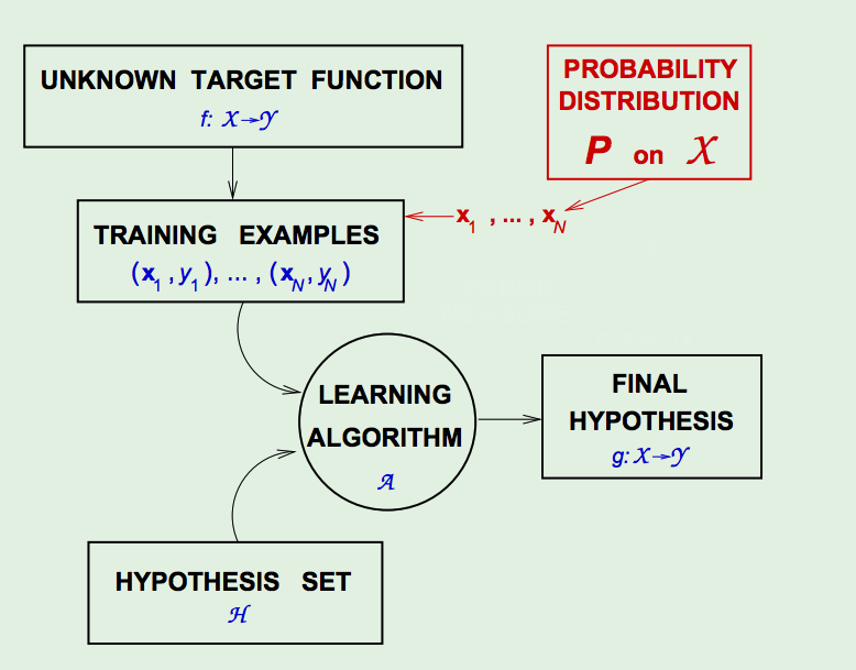
- Error Measures:
Error Measures aim to answer the question:
“What does it mean for \(h\) to approximate \(f\) (\(h \approx f\))?”
The Error Measure: \(E(h, f)\)
It is almost always defined point-wise: \(\mathrm{e}(h(\mathbf{X}), f(\mathbf{X}))\).
Examples:- Square Error: \(\:\:\:\mathrm{e}(h(\mathbf{x}), f(\mathbf{x}))=(h(\mathbf{x})-f(\mathbf{x}))^{2}\)
- Binary Error: \(\:\:\:\mathrm{e}(h(\mathbf{x}), f(\mathbf{x}))=[h(\mathbf{x}) \neq f(\mathbf{x})]\) (1 if true else 0)
The overall error \(E(h,f) =\) average of pointwise errors \(\mathrm{e}(h(\mathbf{x}), f(\mathbf{x}))\):
- In-Sample Error:
$$E_{\mathrm{in}}(h)=\frac{1}{N} \sum_{n=1}^{N} \mathrm{e}\left(h\left(\mathbf{x}_{n}\right), f\left(\mathbf{x}_{n}\right)\right)$$
- Out-Sample Error:
$$E_{\text {out }}(h)=\mathbb{E}_ {\mathbf{x}}[\mathrm{e}(h(\mathbf{x}), f(\mathbf{x}))]$$
- The Learning Diagram - with pointwise error:
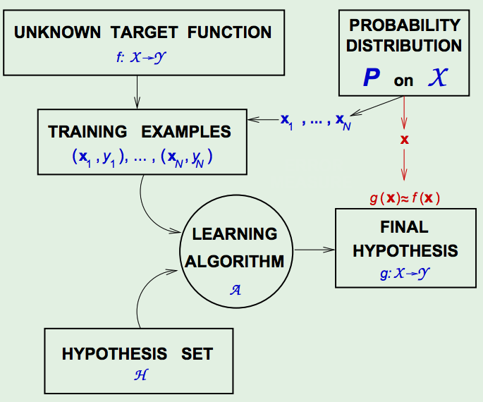
There are two additions to the diagram:- The first is to realize that we are defining the error measure on a point.
- Another is that in deciding whether \(g\) is close to \(f\) , which is the goal of learning, we test this with a point \(x\). And the criterion for deciding whether \(g(x)\) is approximately the same as \(f(x)\) is our pointwise error measure.
-
Defining the Error Measure:
Types:
- False Positive
- False Negative
There is no inherent merit to choosing one error function over another. It’s not an analytic question. It’s an application-domain question.
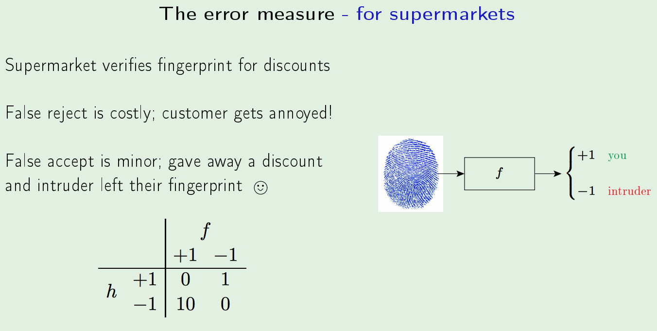
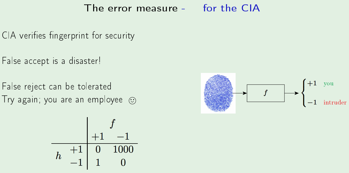
The error measure should be specified by the user. Since, that’s not always possible, the alternatives:
- Plausible Measures: measures that have an analytic argument for their merit, based on certain assumptions.
E.g. Squared Error comes from the Gaussian Noise Assumption. - Friendly Measures: An easy-to-use error measure, without much justification.
E.g. Linear Regression error leads to the easy closed-form solution, Convex Error measures are easy to optimize, etc.
-
The Learning Diagram - with the Error Measure:
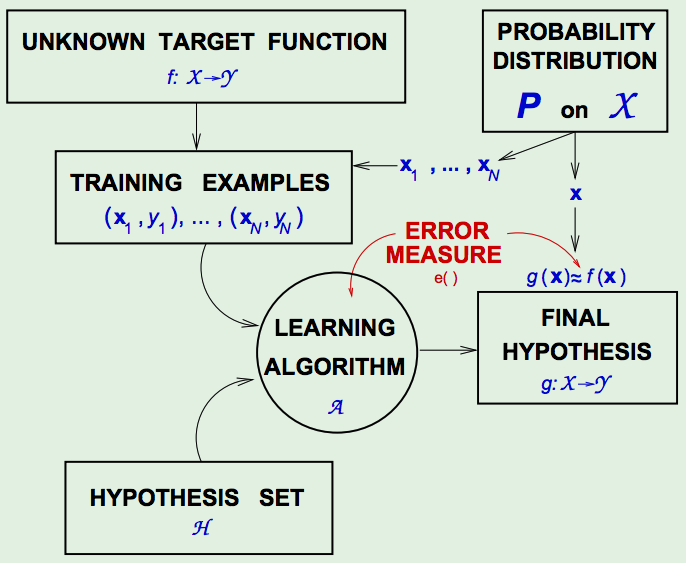
The Error Measure provides a quantitative assessment of the statement \(g(\mathbf{x}) \approx f(\mathbf{x})\). -
Noisy Targets:
The ‘Target Function’ is not always a function because two ‘identical’ input points can be mapped to two different outputs (i.e. they have different labels).The solution: Replacing the target function with a Target Distribution.
Instead of \(y = f(x)\) we use the conditional target distribution: \(P(y | \mathbf{x})\). What changes now is that, instead of \(y\) being deterministic of \(\mathbf{x}\), once you generate \(\mathbf{x}\), \(y\) is also probabilistic– generated by \(P(y | \mathbf{x})\).
\((\mathbf{x}, y)\) is now generated by the joint distribution:$$P(\mathbf{x}) P(y | \mathbf{x})$$
Equivalently, we can define a Noisy Target as a deterministic (target) function \(\:f(\mathbf{x})=\mathbb{E}(y | \mathbf{x})\:\) PLUS Noise \(\: y-f(x)\).
This can be done WLOG since a deterministic target is a special kind of a noisy target:
Define \(P(y \vert \mathbf{x})\) to be identically Zero, except for \(y = f(x)\). -
The Learning Diagram - with the Noisy Target:
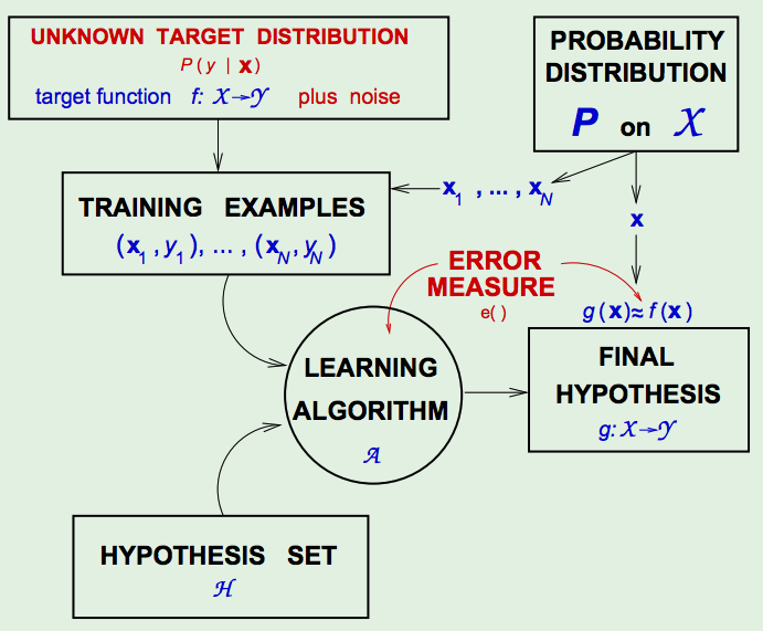
Now, \(E_{\text {out}}(h) = \mathbb{E}_ {x, y}[e(h(x), y)]\) instead of \(\mathbb{E}_ {\mathbf{x}}[\mathrm{e}(h(\mathbf{x}), f(\mathbf{x}))]\), and
\(\left(\mathbf{x}_{1}, y_{1}\right), \cdots,\left(\mathbf{x}_{N}, y_{N}\right)\) are generated independently of each (each tuple). - Distinction between \(P(y | \mathbf{x})\) and \(P(\mathbf{x})\):
The Target Distribution \(P(y \vert \mathbf{x})\) is what we are trying to learn.
The Input Distribution \(P(\mathbf{x})\), only, quantifies relative importance of \(\mathbf{x}\); we are NOT trying to learn this distribution.Rephrasing: Supervised learning only learns \(P(y \vert \mathbf{x})\) and not \(P(\mathbf{x})\); \(P(\mathbf{x}, y)\) is NOT a target distribution for Supervised Learning.
Merging \(P(\mathbf{x})P(y \vert \mathbf{x})\) as \(P(\mathbf{x}, y)\), although allows us to generate examples \((\mathbf{x}, y)\), mixes the two concepts that are inherently different.
- Preamble to Learning Theory:
Generalization VS Learning:
We know that Learning is Feasible.- Generalization:
It is likely that the following condition holds:$$\: E_{\text {out }}(g) \approx E_{\text {in }}(g) \tag{3.1}$$
This is equivalent to “good” Generalization.
- Learning:
Learning corresponds to the condition that \(g \approx f\), which in-turn corresponds to the condition:$$E_{\text {out }}(g) \approx 0 \tag{3.2}$$
How to achieve Learning:
We achieve \(E_{\text {out }}(g) \approx 0\) through:- \(E_{\mathrm{out}}(g) \approx E_{\mathrm{in}}(g)\)
A theoretical result achieved through Hoeffding PROBABILITY THEORY . - \(E_{\mathrm{in}}(g) \approx 0\)
A Practical result of minimizing the In-Sample Error Function (ERM) Optimization .
Learning is, thus, reduced to the 2 following questions:
- Can we make sure that \(E_{\text {out }}(g)\) is close enough to \(E_{\text {in }}(g)\)? (theoretical)
- Can we make \(E_{\text {in}}(g)\) small enough? (practical)
What the Learning Theory will achieve:
- Characterizing the feasibility of learning for infinite \(M\) (hypothesis).
We are going to measure the model not by the number of hypotheses, but by a single parameter which tells us the sophistication of the model. And that sophistication will reflect the out-of-sample performance as it relates to the in-sample performance (through the Hoeffding (then VC) inequalities). - Characterizing the tradeoff:

In words:
We realized that we would like our model, the hypothesis set, to be elaborate, in order to be able to fit the data. The more parameters you have, the more likely you are going to fit the data and get here. So the \(E_{\text{in}}\) goes down if you use more complex models. However, if you make the model more complex, the discrepancy between \(E_{\text{out}}\) and \(E_{\text{in}}\) gets worse and worse. \(E_{\text{in}}\) tracks \(E_{\text{out}}\) much more loosely than it used to.
- Generalization:
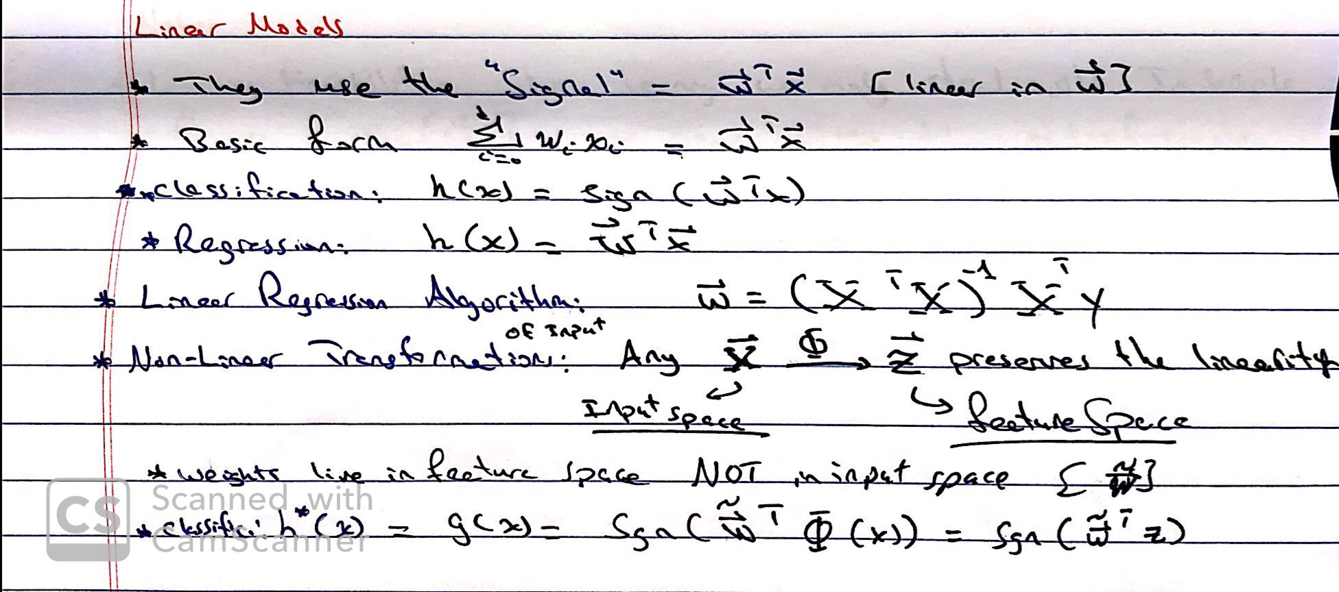
Linear Models I
-
Interpreting Linear Classifiers (cs231n)
- Linear Classifiers Demo (cs231n)
- Linear Regression from Conditional Distribution (gd example)
- Linear Regression Probabilistic Development
- In a linear model, if the errors belong to a normal distribution the least squares estimators are also the maximum likelihood estimators.1
The Linear Model II
- Logistic Regression vs LDA? (ESL)
- Derivation of Logistic Regression
- The Simpler Derivation of Logistic Regression
- Logistic Regression, Generalized Linear and Additive Models (CMU)
- Why do we use the Bernoulli distribution in the logistic regression model? (Quora)
- Logistic Regression - ML Cheatsheet
- Logistic Regression - CS Cheatsheet
- Logistic Regression (Lec Ng)
-
Linear Models - Logistic Regression:
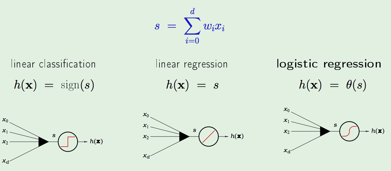
The Logistic Regression applies a non-linear transform on the signal; it’s a softer approximation to the hard-threshold non-linearity applied by Linear Classification. - The Logistic Function \(\theta\):
$$\theta(s)=\frac{e^{s}}{1+e^{s}}=\frac{1}{1+e^{-s}}$$

- Soft Threshold: corresponds to uncertainty; interpreted as probabilities.
- Sigmoid: looks like a flattened out ‘S’.
- The Probability Interpretation:
\(h(\mathbf{x})=\theta(s)\) is interpreted as a probability.
It is in-fact a Genuine Probability. The output of logistic regression is treated genuinely as a probability even during learning.
Justification:
Data \((\mathbf{x}, y)\) with binary \(y\), (we don’t have direct access to probability, but the binary \(y\) is affected by the probability), generated by a noisy target:$$P(y | \mathbf{x})=\left\{\begin{array}{ll}{f(\mathbf{x})} & {\text {for } y=+1} \\ {1-f(\mathbf{x})} & {\text {for } y=-1}\end{array}\right.$$
The target \(f : \mathbb{R}^{d} \rightarrow[0,1]\) is the probability.
We learn \(\:\:\:\: g(\mathbf{x})=\theta\left(\mathbf{w}^{\top} \mathbf{x}\right) \approx f(\mathbf{x})\).In words: So I’m going to call the probability the target function itself. The probability that someone gets heart attack is \(f(\mathbf{x})\). And I’m trying to learn \(f\), notwithstanding the fact that the examples that I am getting are giving me just sample values of \(y\), that happen to be generated by \(f\).
- Logistic Regression uses the sigmoid function to “squash” the output feature/signal into the \([0, 1]\) space.
Although, one could interpret the sigmoid classifier as just a function with \([0,1]\) range, it is actually, a Genuine Probability. - To see this:
- A labeled, classification Data-Set, does NOT (explicitly) give you the probability that something is going to happen, rather, just the fact that an event either happened \((y=1)\) or that it did not \((y=0)\), without the actual probability of that event happening.
- One can think of this data as being generated by a (the following) noisy target:
\({\displaystyle P(y \vert x) ={\begin{cases}f(x)&{\text{for }}y = +1,\\1-f(x)&{\text{for }}y=-1.\\\end{cases}}}\) - They have the form that a certain probability that the event occurred and a certain probability that the event did NOT occur, given their input-data.
- This is generated by the target we want to learn; thus, the function \(f(x)\) is the target function to approximate.
- In Logistic Regression, we are trying to learn \(f(x)\) not withstanding the fact that the data-points we are learning from are giving us just sample values of \(y\) that happen to be generated by \(f\).
- Thus, the Target \(f : \mathbb{R}^d \longrightarrow [0,1]\) is the probability.
The output of Logistic Regression is treated genuinely as a probability even during Learning.
- Logistic Regression uses the sigmoid function to “squash” the output feature/signal into the \([0, 1]\) space.
-
Deriving the Error Measure (Cross-Entropy) from Likelihood:
The error measure for logistic regression is based on likelihood - it is both, plausible and friendly/well-behaved? (for optimization).
For each \((\mathbf{x}, y)\), \(y\) is generated wit probability \(f(\mathbf{x})\).Likelihood: We are maximizing the likelihood of this hypothesis, under the data set that we were given, with respect to the weights. I.E. Given the data set, how likely is this hypothesis? Which means, what is the probability of that data set under the assumption that this hypothesis is indeed the target?
- Deriving the Likelihood:
- We start with:
$$P(y | \mathbf{x})=\left\{\begin{array}{ll}{h(\mathbf{x})} & {\text {for } y=+1} \\ {1-h(\mathbf{x})} & {\text {for } y=-1}\end{array}\right.$$
- Substitute \(h(\mathbf{x})=\theta \left(\mathbf{w}^{\top} \mathbf{x}\right)\):
$$P(y | \mathbf{x})=\left\{\begin{array}{ll}{\theta(\mathbf{w}^T\mathbf{x})} & {\text {for } y=+1} \\ {1-\theta(\mathbf{w}^T\mathbf{x})} & {\text {for } y=-1}\end{array}\right.$$
- Since we know that \(\theta(-s)=1-\theta(s)\), we can simplify the piece-wise function:
$$P(y | \mathbf{x})=\theta\left(y \mathbf{w}^{\top} \mathbf{x}\right)$$
- To get the likelihood of the dataset \(\mathcal{D}=\left(\mathbf{x}_{1}, y_{1}\right), \ldots,\left(\mathbf{x}_{N}, y_{N}\right)\):
$$\prod_{n=1}^{N} P\left(y_{n} | \mathbf{x}_{n}\right) =\prod_{n=1}^{N} \theta\left(y_{n} \mathbf{w}^{\mathrm{T}} \mathbf{x}_ {n}\right)$$
- We start with:
- Maximizing the Likelihood (Deriving the Cross-Entropy Error):
- Maximize:
$$\prod_{n=1}^{N} \theta\left(y_{n} \mathbf{w}^{\top} \mathbf{x}_ {n}\right)$$
- Take the natural log to avoid products:
$$\ln \left(\prod_{n=1}^{N} \theta\left(y_{n} \mathbf{w}^{\top} \mathbf{x}_ {n}\right)\right)$$
Motivation:
- The inner quantity is non-negative and non-zero.
- The natural log is monotonically increasing (its max, is the max of its argument)
- Take the average (still monotonic):
$$\frac{1}{N} \ln \left(\prod_{n=1}^{N} \theta\left(y_{n} \mathbf{w}^{\top} \mathbf{x}_ {n}\right)\right)$$
- Take the negative and Minimize:
$$-\frac{1}{N} \ln \left(\prod_{n=1}^{N} \theta\left(y_{n} \mathbf{w}^{\top} \mathbf{x}_ {n}\right)\right)$$
- Simplify:
$$=\frac{1}{N} \sum_{n=1}^{N} \ln \left(\frac{1}{\theta\left(y_{n} \mathbf{w}^{\tau} \mathbf{x}_ {n}\right)}\right)$$
- Substitute \(\left[\theta(s)=\frac{1}{1+e^{-s}}\right]\):
$$\frac{1}{N} \sum_{n=1}^{N} \underbrace{\ln \left(1+e^{-y_{n} \mathbf{w}^{\top} \mathbf{x}_{n}}\right)}_{e\left(h\left(\mathbf{x}_{n}\right), y_{n}\right)}$$
- Use this as the Cross-Entropy Error Measure:
$$E_{\mathrm{in}}(\mathrm{w})=\frac{1}{N} \sum_{n=1}^{N} \underbrace{\ln \left(1+e^{-y_{n} \mathrm{w}^{\top} \mathbf{x}_{n}}\right)}_{\mathrm{e}\left(h\left(\mathrm{x}_{n}\right), y_{n}\right)}$$
- Maximize:
- Deriving the Likelihood:
- The Decision Boundary of Logistic Regression:
Decision Boundary: It is the set of \(x\) such that:$$\frac{1}{1+e^{-\theta \cdot x}}=0.5 \implies 0=-\theta \cdot x=-\sum_{i=0}^{n} \theta_{i} x_{i}$$
-
The Logistic Regression Algorithm:
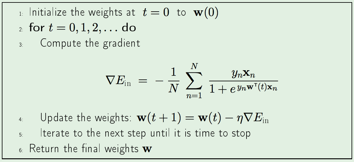
-
Summary of Linear Models:

- Nonlinear Transforms:
$$\mathbf{x}=\left(x_{0}, x_{1}, \cdots, x_{d}\right) \stackrel{\Phi}{\longrightarrow} \mathbf{z}=\left(z_{0}, z_{1}, \cdots \cdots \cdots \cdots \cdots, z_{\tilde{d}}\right)$$
$$\text {Each } z_{i}=\phi_{i}(\mathbf{x}) \:\:\:\:\: \mathbf{z}=\Phi(\mathbf{x})$$
Example: \(\mathbf{z}=\left(1, x_{1}, x_{2}, x_{1} x_{2}, x_{1}^{2}, x_{2}^{2}\right)\)
The Final Hypothesis \(g(\mathbf{x})\) in \(\mathcal{X}\) space:- Classification: \(\operatorname{sign}\left(\tilde{\mathbf{w}}^{\top} \Phi(\mathbf{x})\right)\)
- Regression: \(\tilde{\mathbf{w}}^{\top} \Phi(\mathbf{x})\)
Two Non-Separable Cases:
- Almost separable with some outliers:
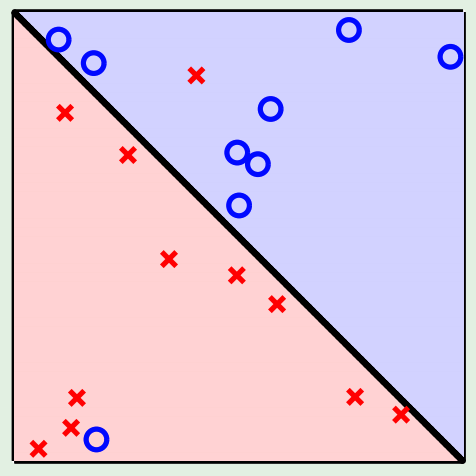
- Accept that \(E_{\mathrm{in}}>0\); use a linear model in \(\mathcal{X}\).
- Insist on \(E_{\mathrm{in}}=0\); go to a high-dimensional \(\mathcal{Z}\).
This has a worse chance for generalizing.
- Completely Non-Linear:
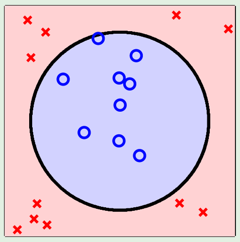
Data-snooping example: it is hard to choose the right transformations; biggest flop is to look at the data to choose the right transformations; it invalidates the VC inequality guarantee.Think of the VC inequality as providing you with a warranty.
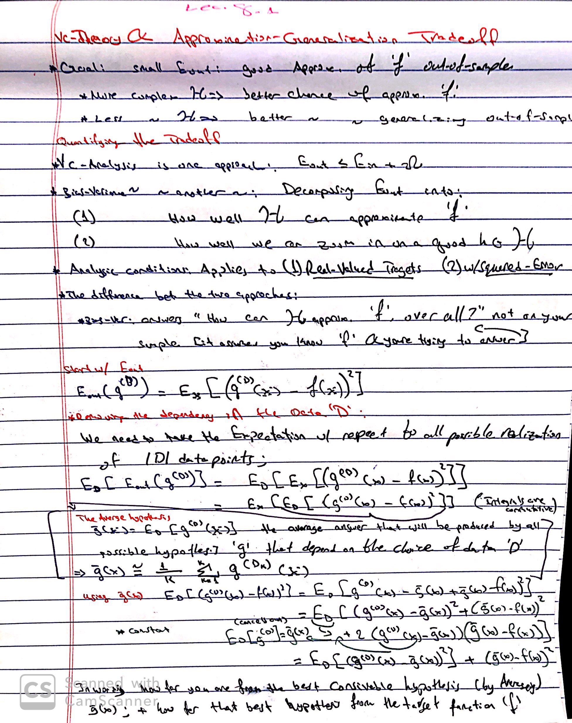
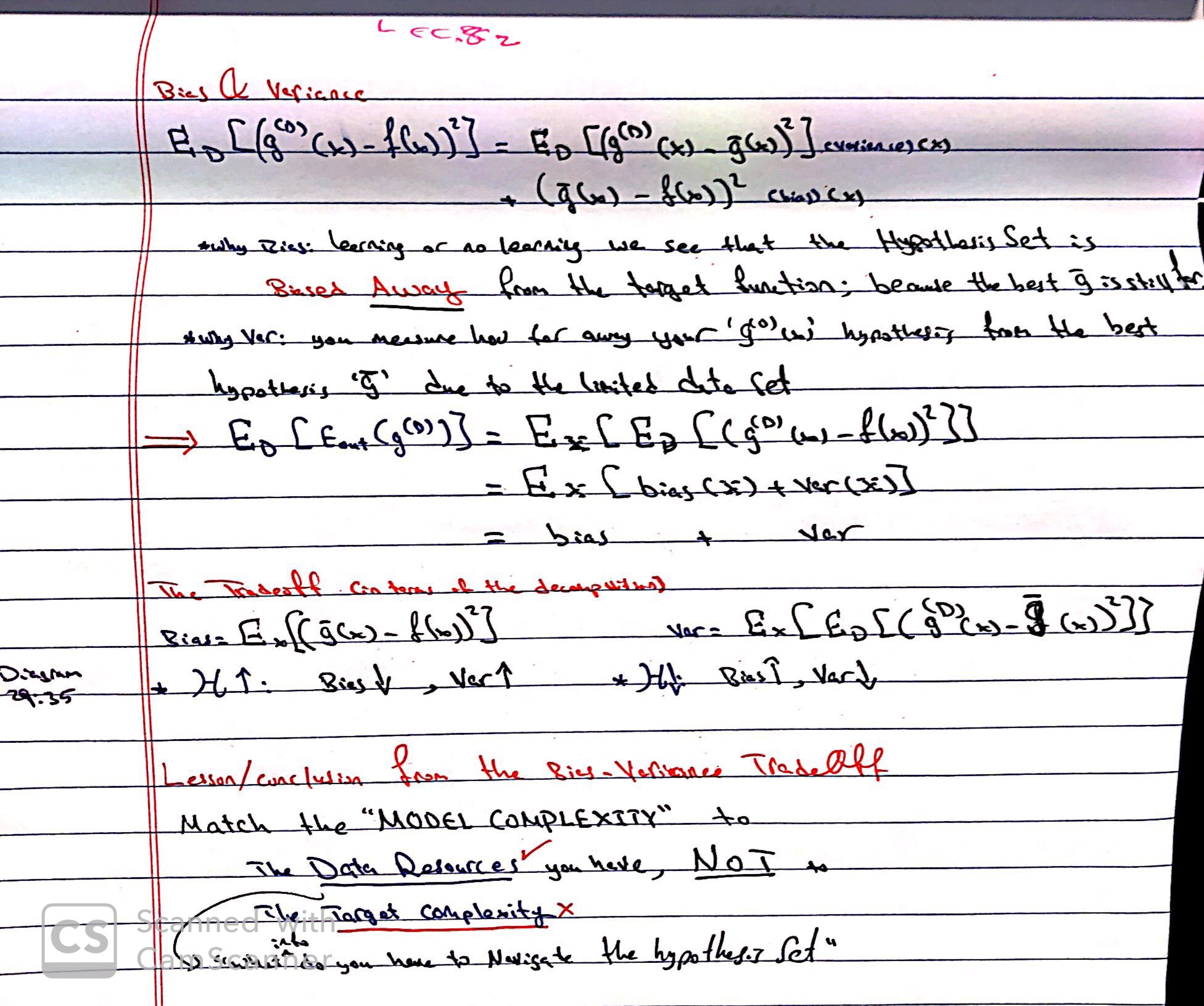
The Bias Variance Decomposition
