Essence of LA - 3b1b
LA (Stanford Review)

Definitions and Intuitions

1. Linear Algebra:
   Linear Algebra is about two operations on a list of numbers:
   1. Scalar Multiplication
   2. Vector Addition
2. Vectors:
   Think of each element in the vector as a scalar that scales the corresponding basis vectors.

   Meaning, think about how each one stretches or squishes vectors (in this case, the basis vectors \(\hat{i}, \hat{j}\))

   $$\begin{bmatrix} x \\ y \end{bmatrix} = \begin{bmatrix} 1 & 0 \\ 0 & 1 \end{bmatrix} \begin{bmatrix} x \\ y \end{bmatrix} = \color{red} x \color{red} {\underbrace{\begin{bmatrix} 1 \\ 0 \end{bmatrix}}_ {\hat{i}}} + \color{red} y \color{red} {\underbrace{\begin{bmatrix} 0 \\ 1 \end{bmatrix}}_ {\hat{j}}} = \begin{bmatrix} 1\times x + 0 \times y \\ 0\times x + 1 \times y \end{bmatrix} $$

3. Span:
   The Span of two vectors \(\mathbf{v}, \mathbf{w}\) is the set of all linear combinations of the two vectors:

   $$a \mathbf{v} + b \mathbf{w} \: ; \: a,b \in \mathbb{R}$$

4. Linearly Dependent Vectors:
   If one vector is in the span of the other vectors.
   Mathematically:

   $$a \vec{v}+b \vec{w}+c \vec{u}=\overrightarrow{0} \implies a=b=c=0$$

5. The Basis:
   The Basis of a vector space is a set of linearly independent vectors that span the full space.

6. Matrix as a Linear Transformation:
   Summary:
   1. Each column is a transformed version of the basis vectors (e.g. \(\hat{i}, \hat{j}\))
   2. The result of a Matrix-Vector Product is the linear combination of the vectors with the appropriate transformed coordinate/basis vectors

      i.e. Matrix-Vector Product is a way to compute what the corresponding linear transformation does to the given vector.

   Matrix as a Linear Transformation:
   Always think of Matrices as Transformations of Space:

   • A Matrix represents a specific linear transformation
     • Where the columns represent the coordinates of the transformed basis vectors
   • & Multiplying a matrix by a vector is EQUIVALENT to Applying the transformation to that vector

     The word “transformation” suggests that you think using movement
     If a transformation takes some input vector to some output vector, we imagine that input vector moving over to the output vector.
     Then to understand the transformation as a whole, we might imagine watching every possible input vector move over to its corresponding output vector.
     This transformation/“movement” is Linear, if it keeps all the vectors parallel and evenly spaced, and fixes the origin.

   Matrices and Vectors | The Matrix-Vector Product:
   Again, We think of each element in a vector as a scalar that scales the corresponding basis vectors.

   • Thus, if we know how the basis vectors get transformed, we can then just scale them (by multiplying with our vector elements).
     Mathematically, we think of the vector:

     $$\mathbf{v} = \begin{bmatrix}x \\y \end{bmatrix} = x\hat{i} + y\hat{j}$$

     and its transformed version:

     $$\text{Transformed } \mathbf{v} = x (\text{Transformed } \hat{i}) + y (\text{Transformed } \hat{j})$$

     \(\implies\) we can describe where any vector \(\mathbf{v}\) go, by describing where the basis vectors will land.

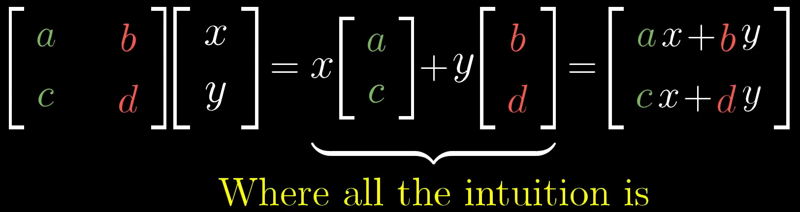
     If you’re given a two-by-two matrix describing a linear transformation and some specific vector and you want to know where that linear transformation takes that vector, you can (1) take the coordinates of the vector (2) multiply them by the corresponding columns of the matrix, (3) then add together what you get.
     This corresponds with the idea of adding the scaled versions of our new basis vectors.
     

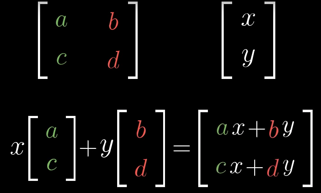
   $$ \mathbf{v} = \begin{bmatrix} x \\ y \end{bmatrix} = \begin{bmatrix} 1 & 0 \\ 0 & 1 \end{bmatrix} \begin{bmatrix} x \\ y \end{bmatrix} = \color{red} x \color{red} {\underbrace{\begin{bmatrix} 1 \\ 0 \end{bmatrix}}_ {\hat{i}}} + \color{red} y \color{red} {\underbrace{\begin{bmatrix} 0 \\ 1 \end{bmatrix}}_ {\hat{j}}} = \begin{bmatrix} 1\times x + 0 \times y \\ 0\times x + 1 \times y \end{bmatrix} = x\hat{i} + y\hat{j} $$

   The Matrix-Vector Product:
   

   Non-Square Matrices \((N \times M)\):
   Map vectors from \(\mathbb{R}^M \rightarrow \mathbb{R}^N\).
   They are transformations between dimensions.

7. The Product of Two Matrices:
   The Product of Two Matrices Corresponds to the composition of the transformations, being applied from right to left.
   This is very important intuition:

   e.g. do matrices commute?
   if you think of the matrices as transformations of space then answer quickly is no.
   Equivalently, Are matrices associative? Yes, function composition is associative (\(f \circ(g \circ h) = (f \circ g) \circ h\))

8. Linear Transformations:
   Linear Transformations are transformations that preserve the following properties:
   1. All vectors that are parallel remain parallel
   2. All vectors are evenly spaced
   3. The origin remains fixed
   • An Equivalent Definition of Linearity

9. The Determinant:
   The Determinant of a transformation is the “scaling factor” by which the transformation changed any area in the vector space.

   The Negative Determinant determines the orientation.

   Linearity of the Determinant:

   $$\text{det}(AB) = \text{det}(A) \text{det}(B)$$

10. Solving Systems of Equations:
    The Equation \(A\mathbf{x} = \mathbf{b}\), finds the vector \(\mathbf{x}\) that lands on the vector \(\mathbf{b}\) when the transformation \(A\) is applied to it.

    Again, the intuition: is to think of a linear system of equations, geometrically, as trying to find a particular vector that once transformed/moved, lands on the output vector \(\mathbf{b}\).

    • This becomes more important when you think of the different properties, of that transformation/function, encoded (now) in the matrix \(A\):
      • When the \(det(A) \neq 0\) we know that space is preserved, and from the properties of linearity, we know there will always be one (unique) vector that would land on \(\mathbf{b}\) once transformed (and you can find it by “playing the transformation in reverse” i.e. the inverse matrix).
      • When \(det(A) = 0\) then the space is squished down to a lower representation, resulting in information loss.

11. The Inverse of a matrix:
    The Inverse of a matrix is the matrix such that if we “algebraically” multiply the two matrices, we get back to the original coordinates (the identity).
    It is, basically, the transformation applied in reverse.

    Why inverse transformation/matrix DNE when det is Zero (i.e. space is squished:
    To do so, is equivalent to transforming a line into a plane, which would require mapping each, individual, vector into a “whole line full of vectors” (multiple vectors); which is not something a Function can do.
    Functions map single input to single output.

12. The Determinants, Inverses, & Solutions to Equations:
    When the \(\text{det} = 0\) the area gets squashed to \(0\), and information is lost. Thus:
    1. The Inverse DNE
    2. A unique solution DNE

       i.e. there is no function that can take a line onto a plane; info loss

13. The Rank:
    The Rank is the dimensionality of the output of a transformation.
    Viewed as a Matrix, it is the number of independent vectors (as columns) that make up the matrix.

14. The Column Space:
    The Column Space is the set of all possible outputs of a transformation/matrix.
    • View each column as a basis vector; there span is then, all the possible outputs
    • The Zero Vector (origin): is always in the column space (corresponds to preserving the origin)

    The Column Space allows us to understand when a solution exists.
    For example, even when the matrix is not full-rank (det=0) a solution might still exist; if, when \(A\) squishes space onto a line, the vector \(\mathbf{b}\) lies on that line (in the span of that line).

    • Formally, solution exists if \(\mathbf{b}\) is in the column space of \(A\).

15. The Null Space:
    The Null Space is the set of vectors that get mapped to the origin; also known as The Kernel.

    The Null Space allows us to understand what the set of all possible solutions look like.

    Rank and the Zero Vector:
    A Full-Rank matrix maps only the origin to itself.
    A non-full rank (det=0) (rank=n-1) matrix maps a whole line to the origin, (rank=n-2) a plane to the origin, etc.

16. The Dot Product/Scalar Product:
    (for vectors \(\mathbf{u}, \mathbf{v}\))

    $$\mathbf{u} \cdot \mathbf{v} = \mathbf{u}^T \mathbf{v}$$

    • Geometrically:
      1. project
17. Cramer’s Rule:
    • Cramer’s Rule Geometrically

18. Coordinate Systems:

    A Coordinate System is just a way to formalize the basis vectors and their lengths. All coordinate systems agree on where the origin is.
    Coordinate Systems are a way to translate between vectors (defined w.r.t. basis vectors being scaled and added in space) and sets of numbers (the elements of the vector/list/array of numbers which we define).

    • Translating between Coordinate Systems

      Imp: 6:47

    • Translating a Matrix/Transformation between Coordinate Systems

    Implicit Assumptions in a Coordinate System:

    • Direction of each basis vector our vector is scaling
    • The unit of distance

19. Eigenstuff:

    • Computing the Eigenvalues/vectors Intuition
    • Diagonalization

    Notes:

    • Complex Eigenvalues, generally, correspond to some kind of rotation in the transformation/matrix (think, multiplication by \(i\) in \(\mathbb{C}\) is a \(90^{\deg}\) rotation).
    • For a diagonal matrix, all the basis vectors are eigenvectors and the diagonal entries are their eigenvalues.