Table of Contents
Full Treatment of Naive Bayes Classification
Bayes Classifier and Bayes Error (paper)
Bayes Classifier and Bayes Error (question)
Naive Bayes CS188 (+Probabilistic Calibration)

A Naive Bayes classifier that figured out that you liked pickles and ice cream would probably naively recommend you a pickle ice cream.
Introduction and the Naive Bayes Classifier
-
Naive Bayes:
Naive Bayes is a simple technique for constructing classifiers. -
Naive Bayes Classifiers:
Naive Bayes Classifiers are a family of simple probabilistic classifiers based on applying Bayes’ Theorem with strong (naive) independence assumptions between the features.The Assumptions:
- Naive Independence: the feature probabilities are indpendenet given a class \(c\).
- Bag-of-Words: we assume that the position of the words does not matter.
Notes:
- Not a Bayesian Method: the name only references the use of Bayes’ theorem in the classifier’s decision rule
- The Naive Bayes Classifier is a Bayes Classifier (i.e. minimizes the prob of misclassification)
- As a Parametric Model (analysis):
- A Bayes classifier basically picks the label \(y\) that has the maximum probability, given that testing data-point \(x\):
\(y^{* }=\operatorname{argmax}_ {y} P(y)=\operatorname{argmax}_ {y} \frac{P(x \mid y) P(y)}{P(x)}\)
If you assume the features of \(x\) are conditionally independent given the label, you get the Naive Bayes classifier.
So, classification depends a lot on \(P(x \mid y)\). The parametric way to classify would be to decide a model (Gaussian, Bernoulli, etc.) for the features of \(x\), and typically the models are different for different classes \(y\). The parameters here are the parameters of your model (mean and covariance for Gaussian, individual feature probabilities for Bernoulli, etc.) and the training problem becomes a parameter estimation problem.
- A Bayes classifier basically picks the label \(y\) that has the maximum probability, given that testing data-point \(x\):
- The Probabilistic Model (Naive Bayes Probability/Statistical Model):
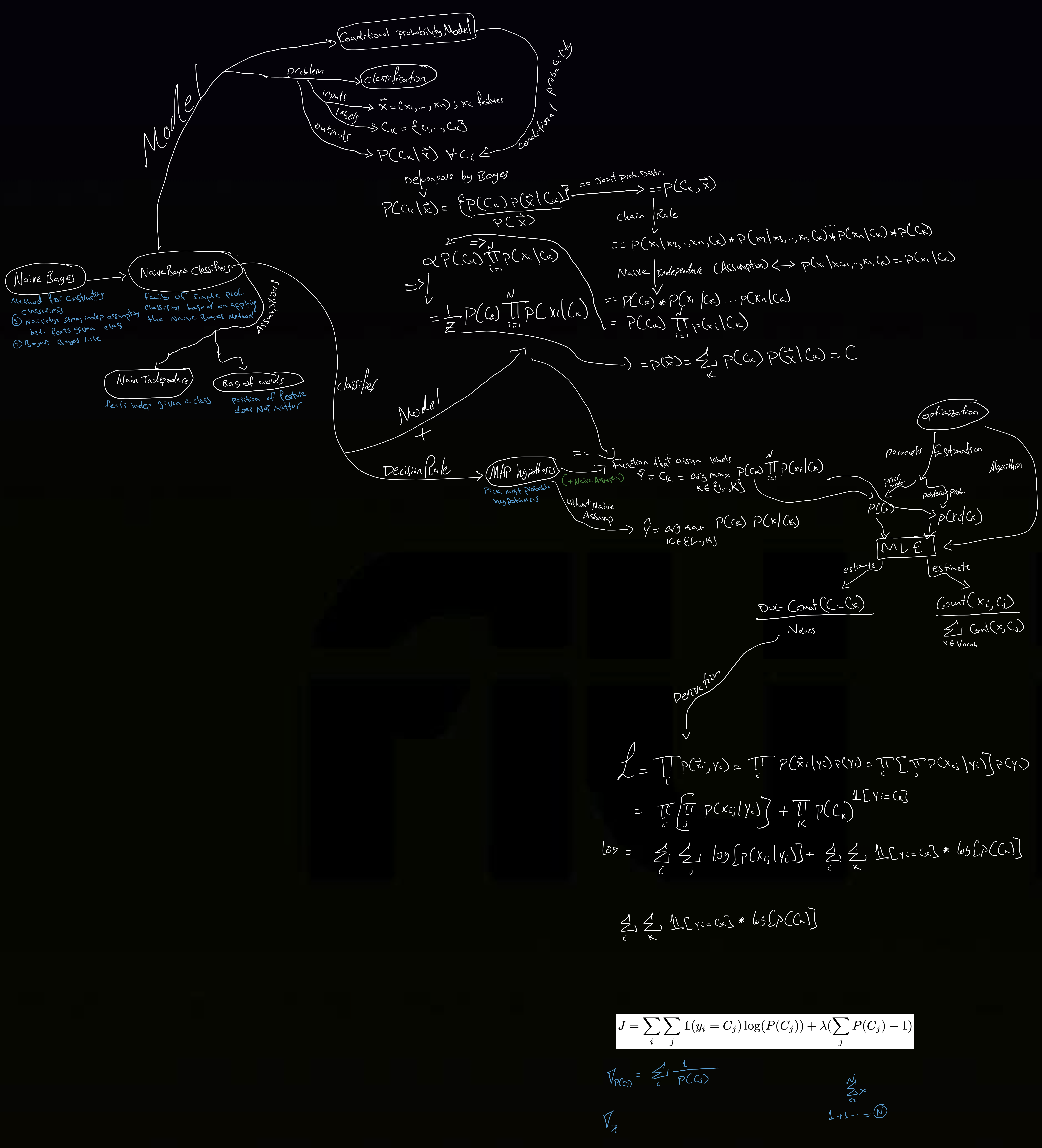
Abstractly, naive Bayes is a conditional probability model:
given a problem instance to be classified, represented by a vector \({\displaystyle \: \mathbf{x} =(x_{1},\dots ,x_{n})}\) representing some \(n\) features (independent variables), it assigns to this instance probabilities$${\displaystyle p(C_{k}\mid x_{1},\dots ,x_{n}) = p(C_{k}\mid \mathbf {x})}$$
for each of the \(k\) possible classes \(C_k\).
Using Bayes’ Theorem we decompose the conditional probability as:
$${\displaystyle p(C_{k}\mid \mathbf {x} )={\frac {p(C_{k})\ p(\mathbf {x} \mid C_{k})}{p(\mathbf {x} )}}\,}$$
Notice that the numerator is equivalent to the joint probability distribution:
$$p\left(C_{k}\right) p\left(\mathbf{x} | C_{k}\right) = p\left(C_{k}, x_{1}, \ldots, x_{n}\right)$$
Using the Chain-Rule for repeated application of the conditional probability, the joint probability model can be rewritten as:
$$p(C_{k},x_{1},\dots ,x_{n})\, = p(x_{1}\mid x_{2},\dots ,x_{n},C_{k})p(x_{2}\mid x_{3},\dots ,x_{n},C_{k})\dots p(x_{n-1}\mid x_{n},C_{k})p(x_{n}\mid C_{k})p(C_{k})$$
Using the Naive Conditional Independence assumptions:
$$p\left(x_{i} | x_{i+1}, \ldots, x_{n}, C_{k}\right)=p\left(x_{i} | C_{k}\right)$$
Thus, we can write the joint model as:
$${\displaystyle {\begin{aligned}p(C_{k}\mid x_{1},\dots ,x_{n})&\varpropto p(C_{k},x_{1},\dots ,x_{n})\\&=p(C_{k})\ p(x_{1}\mid C_{k})\ p(x_{2}\mid C_{k})\ p(x_{3}\mid C_{k})\ \cdots \\&=p(C_{k})\prod _{i=1}^{n}p(x_{i}\mid C_{k})\,,\end{aligned}}}$$
Finally, the conditional distribution over the class variable \(C\) is:
$${\displaystyle p(C_{k}\mid x_{1},\dots ,x_{n})={\frac {1}{Z}}p(C_{k})\prod _{i=1}^{n}p(x_{i}\mid C_{k})}$$
where, \({\displaystyle Z=p(\mathbf {x} )=\sum _{k}p(C_{k})\ p(\mathbf {x} \mid C_{k})}\) is a constant scaling factor,dependent only on the, known, feature variables \(x_i\)s.
-
The Classifier:
We can construct the classifier from the probabilistic model above.
The Naive Bayes Classifier combines this model with a decision rule.The Decision Rule:
we commonly use the Maximum A Posteriori (MAP) hypothesis, as the decision rule; i.e. pick the hypothesis that is most probable.The Classifier is the function that assigns a class label \(\hat{y} = C_k\) for some \(k\) as follows:
$${\displaystyle {\hat {y}}={\underset {k\in \{1,\dots ,K\}}{\operatorname {argmax} }}\ p(C_{k})\displaystyle \prod _{i=1}^{n}p(x_{i}\mid C_{k}).}$$
It, basically, maximizes the probability of the class given an input \(\boldsymbol{x}\).
- Naive Bayes Estimate VS MAP Estimate:
MAP Estimate:$${\displaystyle {\hat {y}_{\text{MAP}}}={\underset {k\in \{1,\dots ,K\}}{\operatorname {argmax} }}\ p(C_{k})\ p(\mathbf {x} \mid C_{k})}$$
Naive Bayes Estimate:
$${\displaystyle {\hat {y}_{\text{NB}}}={\underset {k\in \{1,\dots ,K\}}{\operatorname {argmax} }}\ p(C_{k})\displaystyle \prod _{i=1}^{n}p(x_{i}\mid C_{k})}$$
- Estimating the Parameters of the Classifier:
Parameters to be Estimated:- The prior probability of each class:
$$p(C_{k})$$
- The conditional probability of each feature (word) given a class:
$$p(x_{i}\mid C_{k}) \:\: \forall i \in {1, .., n}$$
We, generally, use Maximum Likelihood Estimates for the parameters.
The MLE Estimates for the Parameters:
- \(\hat{P}(C_k) = \dfrac{\text{doc-count}(C=C_k)}{N_\text{doc}}\),
- \(\hat{P}(x_i | C_j) = \dfrac{\text{count}(x_i,C_j)}{\sum_{x \in V} \text{count}(x, C_j)}\)
- The prior probability of each class:
- MLE Derivation of the Parameter Estimates:
The Likelihood of the observed data (TBC)
-
Motivation:
To estimate the parameters of the “true” MAP estimate, we need a prohibitive number of examples ~ \(\mathcal{O}(\vert x\vert^n \cdot \vert C\vert)\). - Notes:
- In a naive Bayes classifier we are interested in computing the conditional \(p(y \mid x ; \theta) \propto p(y ; \theta) \prod_{i}^{d} p\left(x_{i} \mid y ; \theta\right)\).
Is this a parametric or nonparametric model? The model is specified by \(\mathcal{H}=\{p(x, y ; \theta)\}\) where \(\theta\) contains the parameter for the class prior multinomial distribution \(p(y)\) (finite number of parameters), and the class conditional distributions \(p\left(x_{i} \mid y\right)\) for each dimension. The latter can be parametric (such as a multinomial over the vocabulary, or a Gaussian), or nonparametric (such as \(1D\) kernel density estimation). Therefore, naive Bayes can be either parametric or nonparametric, although in practice the former is more common.
In machine learning we are often interested in a function of the distribution \(T(F)\), for example, the mean. We call \(T\) the statistical functional, viewing \(F\) the distribution itself a function of \(x\). However, we will also abuse the notation and say \(\theta=T(F)\) is a “parameter” even for nonparametric models.
- In a naive Bayes classifier we are interested in computing the conditional \(p(y \mid x ; \theta) \propto p(y ; \theta) \prod_{i}^{d} p\left(x_{i} \mid y ; \theta\right)\).