Algebraic Polynomials

1. Fundamental Theorem of Algebra:
   

2. Existance of Roots:
   

3. Polynomial Equivalence:
   

   This result implies that to show that two polynomials of degree less than or equal to \(n\) are the same, we only need to show that they agree at \(n + 1\) values.

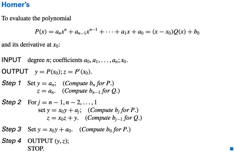
Horner’s Method

1. What?
   Horner’s method incorporates the Section 1.2 nesting technique, and, as a consequence, requires only n multiplications and n additions to evaluate an arbitrary nth-degree polynomial.

2. Why?
   To use Newton’s method to locate approximate zeros of a polynomial P(x), we need to evaluate \(P(x)\) and \(P'(x)\) at specified values, Which could be really tedious.

3. Horner’s Method:
   
   

4. Algorithm:
   

5. Horner’s Derivatives:
   

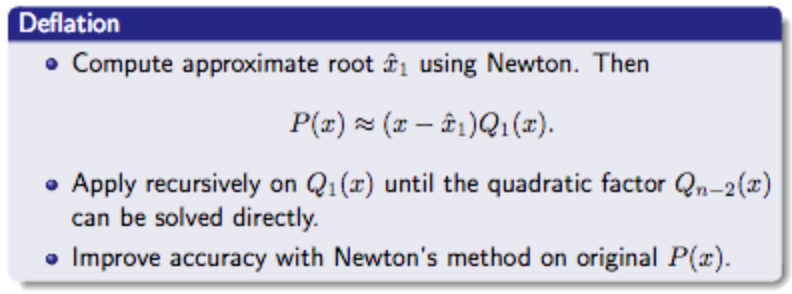
6. Deflation:
   

7. MatLab Implementation:
   

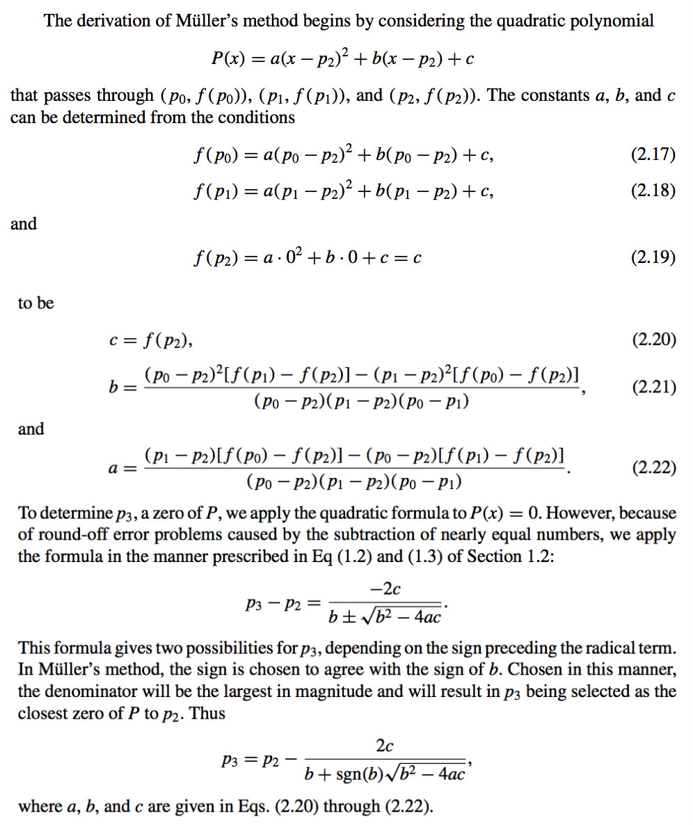
Complex Zeros: Müller’s Method

1. What?
   
   • A synthetic division involving quadratic polynomials can be devised to approximately factor the polynomial so that one term will be a quadratic polynomial whose complex roots are approximations to the roots of the original polynomial
   • Müller’s method uses three initial approximations, \(p_0, p_1,\) and \(p_2\), and determines the next approximation \(p_3\) by considering the intersection of the x-axis with the parabola through \(( p_0,\ f ( p_0)), \ \ ( p_1,\ f ( p_1))\), and \(\ \ ( p_2,\ f ( p_2))\)

   Derivation can be found here!

2. Why?
   

   Newton’s Method/Secant/False Postion Weakness: The possibility that the polynomial having complex roots even when all the coefficients are real numbers.

   If the initial approximation is a real number, all subsequent approximations will also be real numbers.

3. Complex Roots:
   

4. Algorithm:
   Show Algorithm

5. Calculations and Evaluations:
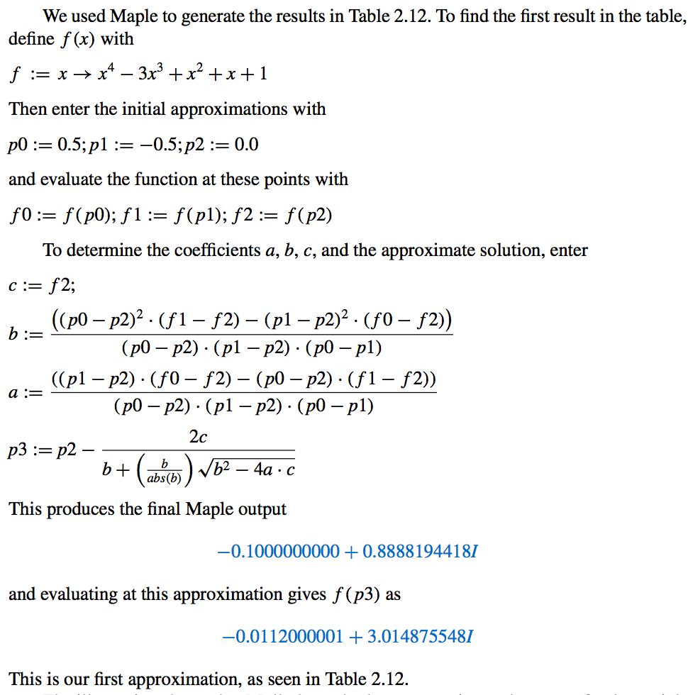
   HERE!

   Müller’s method can approximate the roots of polynomials with a variety of starting values.