Table of Contents
Main Idea
-
- What?
-
- Efficient techniques for calculating integrals in intervals with high functional variations.
- They predict the amount of functional variation and adapt the step size as necessary.
-
- Why?
- The composite formulas suffer because they require the use of equally-spaced nodes.
This is inappropriate when integrating a function on an interval that contains both regions with large functional variation and regions with small functional variation.
-
- Approximation Formula:
- \(\int_{a}^{b} f(x) dx =\)
-
- Error Bound:
- Error relative to Composite Approximations:
- Error relative to True Value:
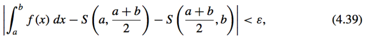
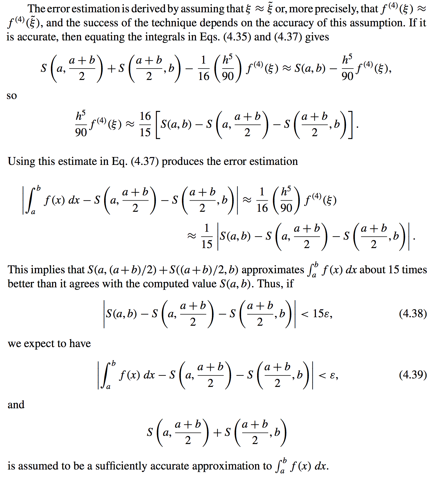
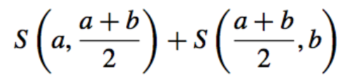
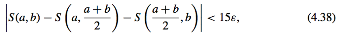
This implies that this procedure approximates the integral about 15 times better than it agrees with the computed value \(S(a, b)\).
- Error relative to Composite Approximations:
- Procedure:
When the approximations in (4.38) differ by more than \(15\epsilon\), we can apply the Simpson’s rule technique individually to the subintervals \([a,\dfrac{a + b}{2}]\) and \([\dfrac{a + b}{2}, b]\).
Then we use the error estimation procedure to determine if the approximation to the integral on each subinterval is within a tolerance of \(\epsilon/2\). If so, we sum the approximations to produce an approximation to \(\int_{a}^{b} f(x) dx\), within the tolerance \(\epsilon\).
If the approximation on one of the subintervals fails to be within the tolerance \(\epsilon/2\), then that subinterval is itself subdivided, and the procedure is reapplied to the two subintervals to determine if the approximation on each subinterval is accurate to within \(\epsilon/4\). This halving procedure is continued until each portion is within the required tolerance.
-
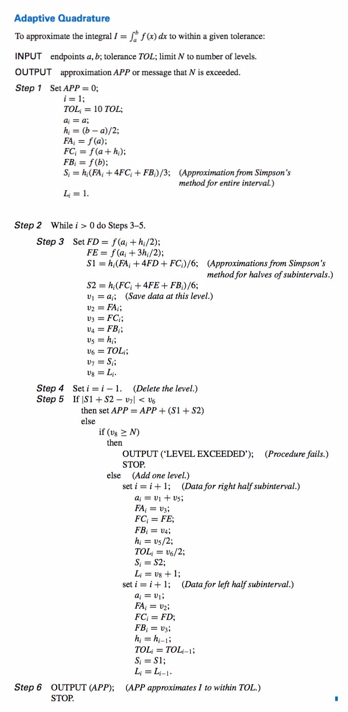
Algorithm:
- Derivation: