Table of Contents
Approximating Double Integral
-
- What?
- The techniques discussed in the previous sections can be modified for use in the approximation of multiple integrals.
-
Why?
-
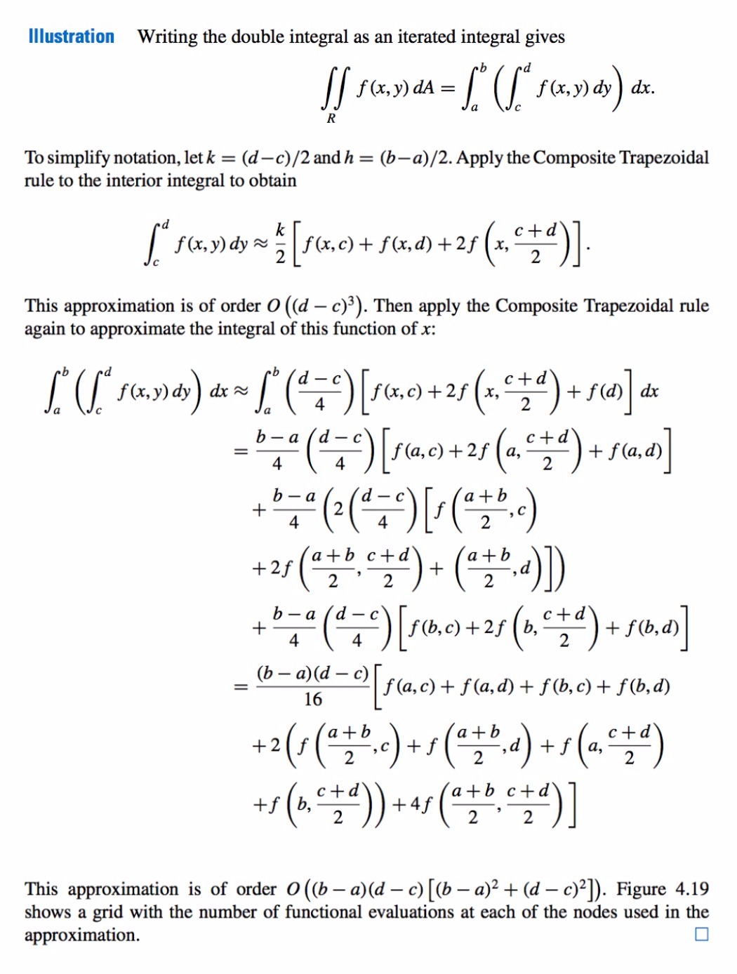
Comoposite Trapezoidal Rule for Double Integral:
\(\ \ \iint_R f(x,y) \,dA \ = \ \int_{a}^{b} \ \big( \ \int_{c}^{d} \ \ f(x,y) \ \ dy \ \ \big) \ dx \ \ \\)\(\approx \dfrac{(b − a)(d − c)}{16} \bigg[f(a,c)+f(a,d) + f(b,c) + f(b,d)+\) \(\ \ \ \ \ \ \ \ 2\Big[f\big(\dfrac{a + b}{2} , c\big) + f\big(\dfrac{a + b}{2} , d\big) + f\big(a, \dfrac{c + d}{2}\big) + f\big(b, \dfrac{c + d}{2}\big)\Big] + 4f\big(\dfrac{a + b}{2}, \dfrac{c + d}{2}\big)\bigg]\)
- Comoposite Simpsons’ Rule for Double Integral:
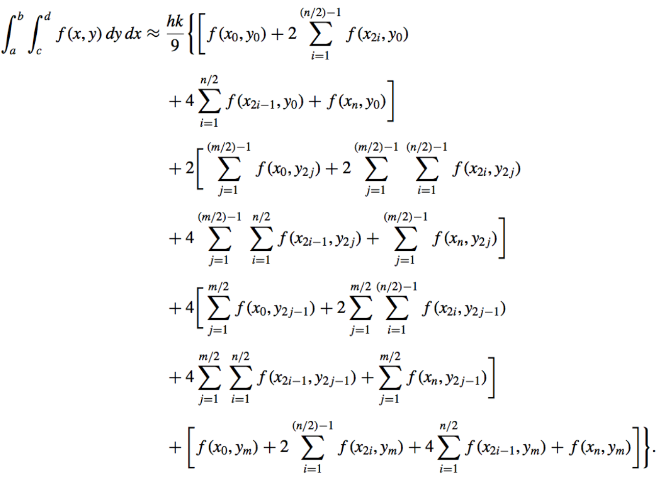
- Rule:
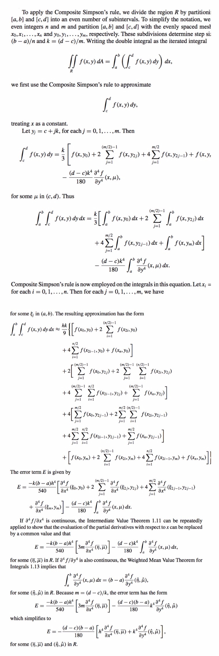
- Error:

- Derivation:
- Rule:
Gaussian Quadrature for Double Integral Approximation
-
- What?
- More efficient methods such as Gaussian quadrature, Romberg integration, or Adaptive quadrature can be incorporated in place of the Newton-Cotes formulas.
-
- Why?
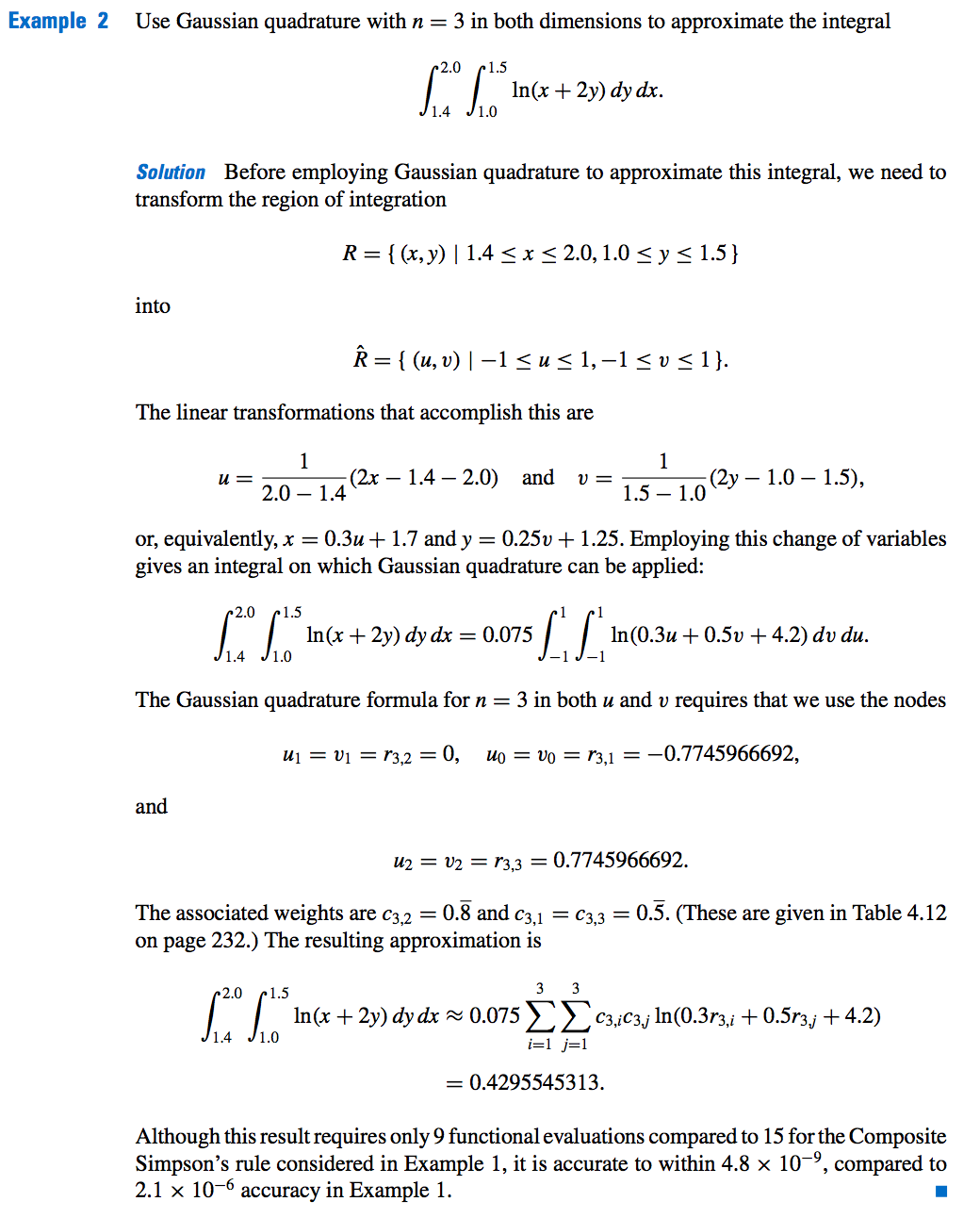
- To reduce the number of functional evaluations.
- Example:
Non-Rectangular Regions
-
- What?
- Regions that don’t have a rectangular shape.
- Form:
- \[\ \int_{a}^{b} \bigg( \int_{c(x)}^{d(x)} f(x,y) dy \bigg) dx \ \ \ \ \ \ \ \ \ \ \ \ \ \ \ \ \ \ \ \ \ \ \ \ \ \ \ \ \ \ \ \ \ \ \ \ \ \ \ \ \ \ \ \ \ \ \ \ \ \ \ \ (4.42)\]
- or,
- \[\int_{c}^{d} \bigg( \int_{a(y)}^{b(y)} f(x,y) dx \bigg) dy \ \ \ \ \ \ \ \ \ \ \ \ \ \ \ \ \ \ \ \ \ \ \ \ \ \ \ \ \ \ \ \ \ \ \ \ \ \ \ \ \ \ \ \ \ \ \ \ \ \ \ \ \ (4.43)\]
- How?
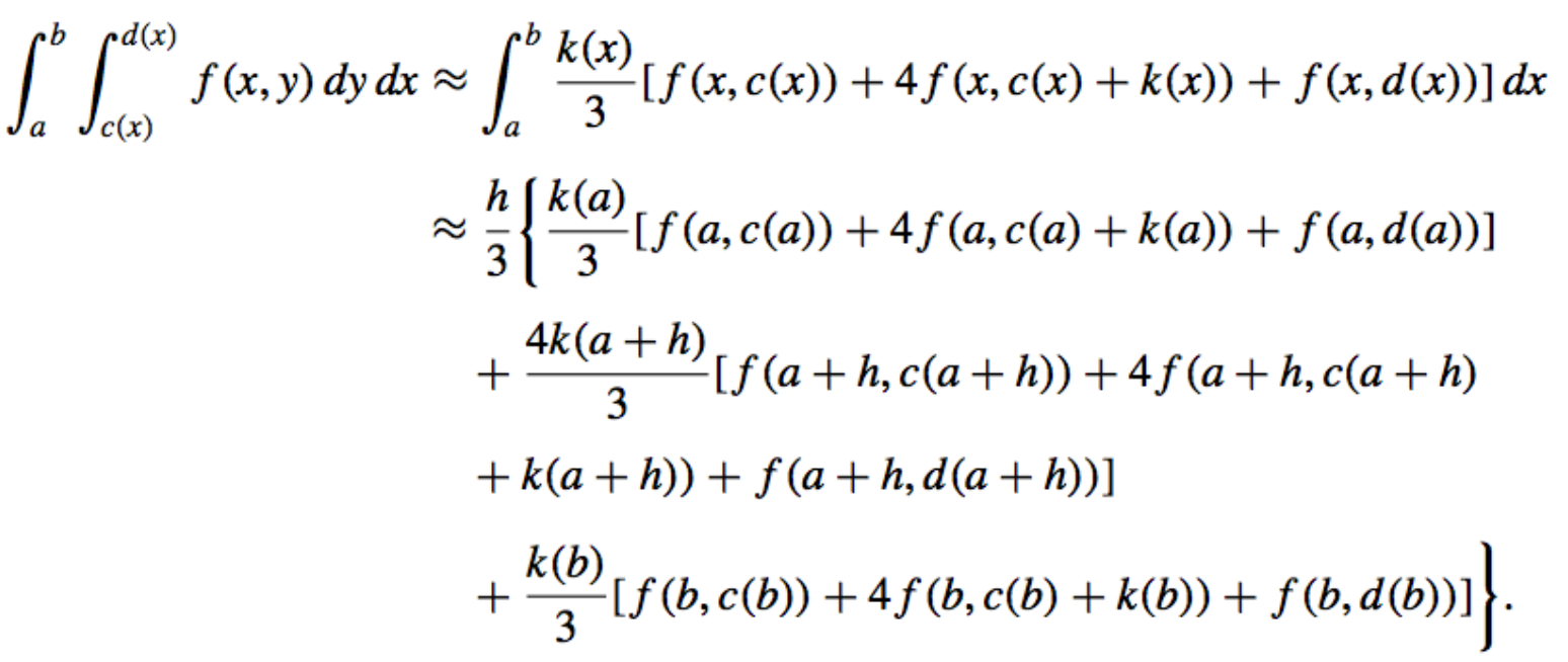
- We use Simpson’s Rule for Approximation.
- Step Size:
- x: \(\ \ h = \dfrac{b − a}{2}\)
- y: \(\ \ k(x) = \dfrac{d(x) − c(x)}{2}\)
- Simpsons’ Rule for Non-Rect Regions:
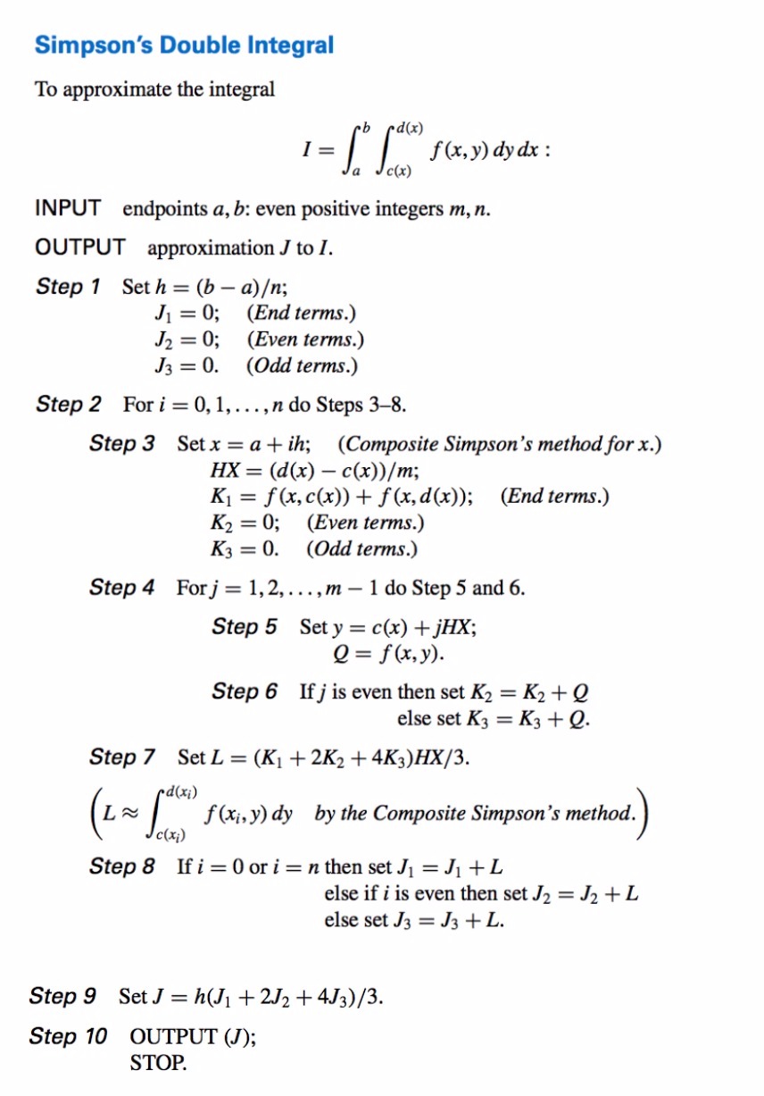
- Simpsons’ Double Integral [Algorithm]:
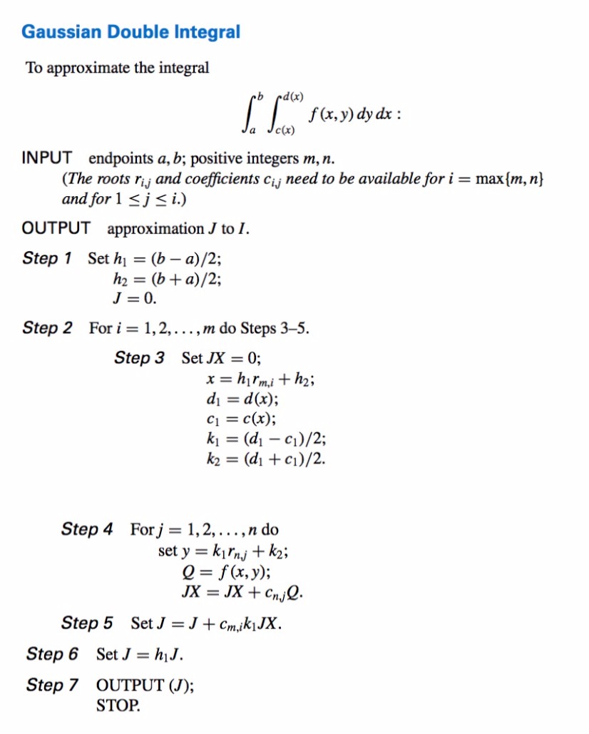
- Gaussian Double Integral [Algorithm]:
Triple Integral Approximation
-
- What?
-
- Triple integrals.
-
- Form:
- \[\ \int_{a}^{b} \ \int_{c(x)}^{d(x)} \ \int_{\alpha(x)}^{\beta(x)} f(x,y) dz \ dy \ dx\]
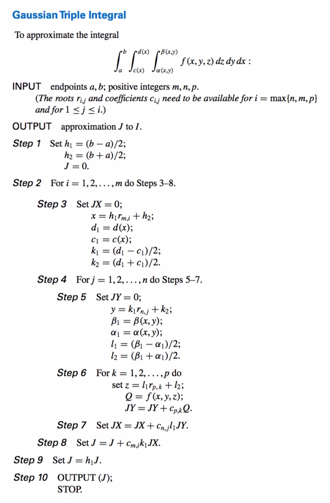
- Gaussian Triple Integral [Algorithm]:
