Eulers Method
-
- What?
-
- The object of Euler’s method is to obtain approximations to the well-posed initial-value problem
\(\ \ \ \ \ \ \ \ \ \ \ \ \ \ \ \ \dfrac{dy}{dt} = f(t,y), \ \ \ \ \ \ a \leq b, \ \ \ \ \ \ y(a) = \alpha \ \ \ \ \ \ \ \ \ \ \ \ \ \ \ \ \ \ \ \ \ \ \ \ \ \ \ \ \ \ \ \ \ \ \ \ \ \ \ \ \ \ \ \ (5.6)\)
- The object of Euler’s method is to obtain approximations to the well-posed initial-value problem
-
- A continuous approximation to the solution \(y(t)\) will not be obtained; instead, approximations to \(y\) will be generated at various values, called mesh points, in the interval \([a, b]\).
-
- Once the approximate solution is obtained at the points, the approximate solution at other points in the interval can be found by interpolation.
-
- Mesh-Points:
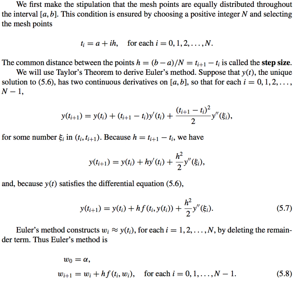
- \[t_i = a + ih, \ \ \ \text{for each } i = 0, 1, 2, ... , N\]
-
The mesh points are equally distributed throughout the interval \([a, b]\).
-
- Step-Size:
- \[h = \dfrac{b − a}{N} = t_{i+1} − t\]
-
Euler’s Method:
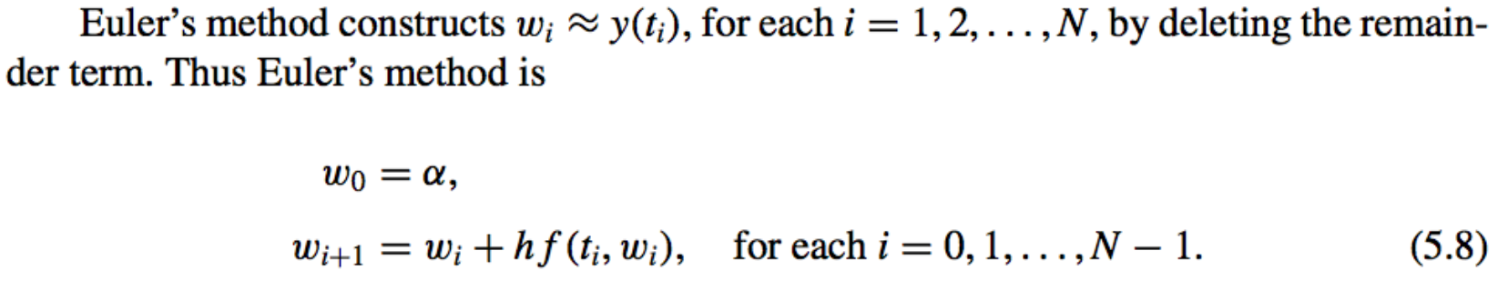
Equation \((5.8)\) is called the difference equation associated with Euler’s method.
-
Derivation:
-
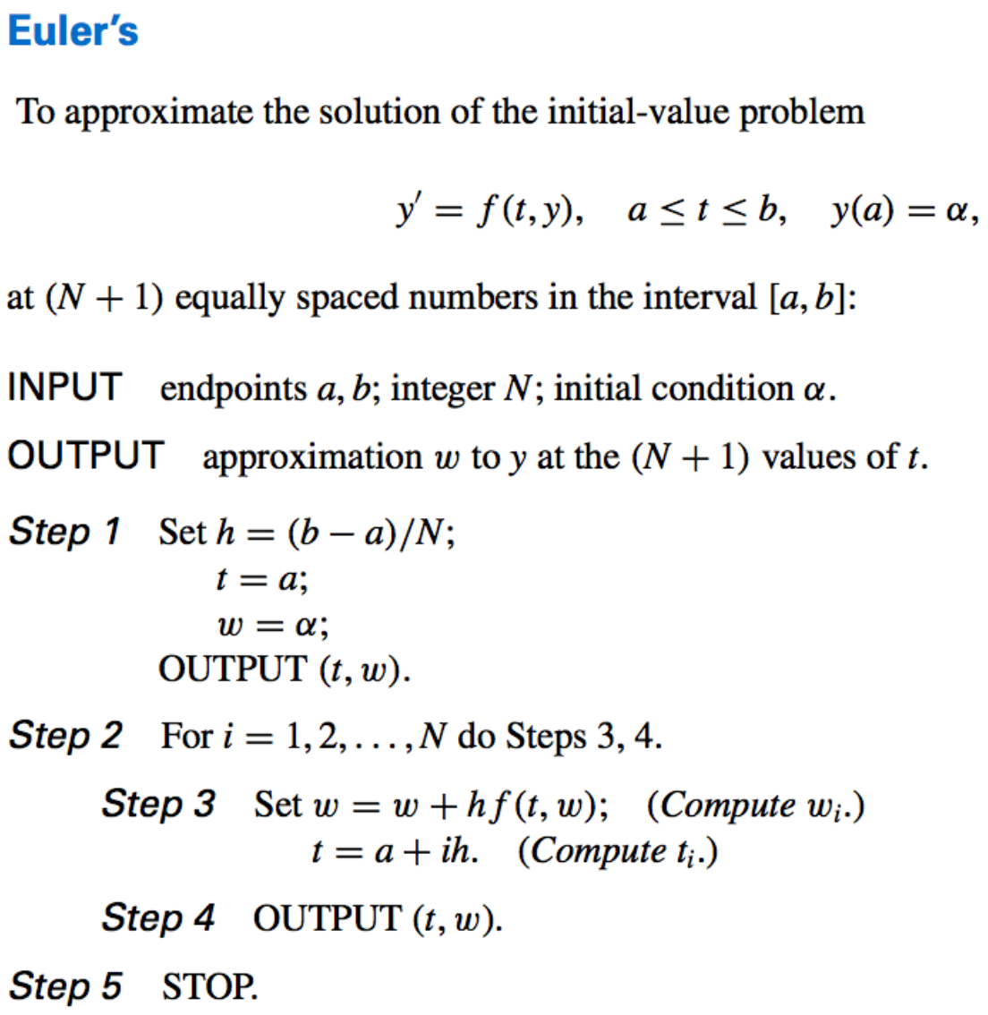
Algorithm:
- Geometric Interpetation:
To interpret Euler’s method geometrically, note that when \(w_i\) is a close approximation to \(y(t_i)\), the assumption that the problem is well-posed implies that \(f(t_i, w_i) \approx y(t_i) = f(t_i, y(t_i))\).i.e. each step corresponds to correcting the path by the approximation to the derivative (slope).
Error Bounds for Euler’s Method
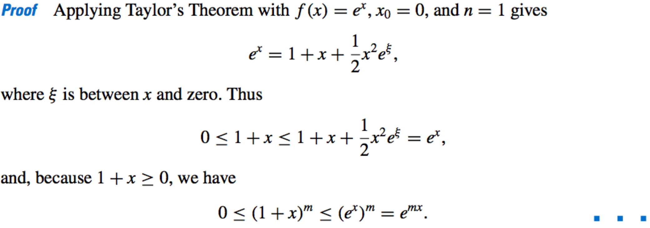
- Comparison Lemmas:
-
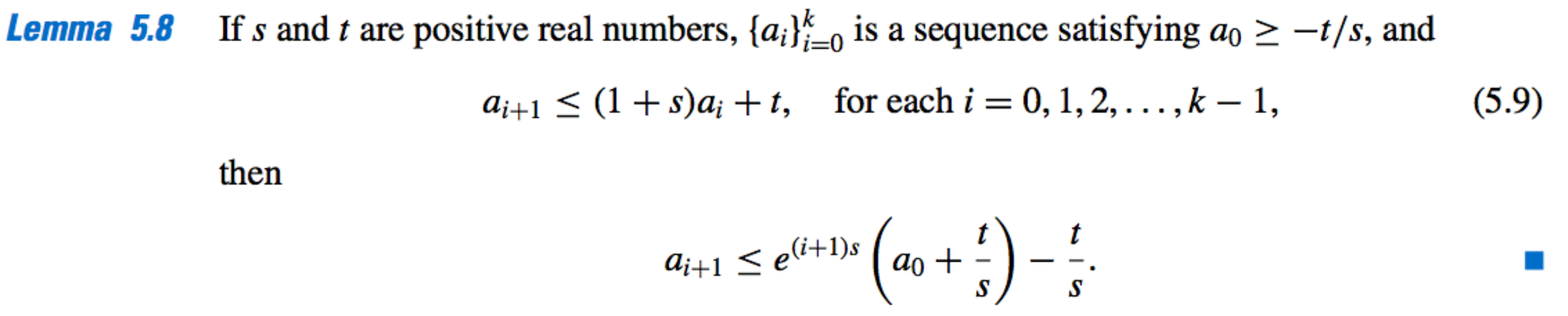
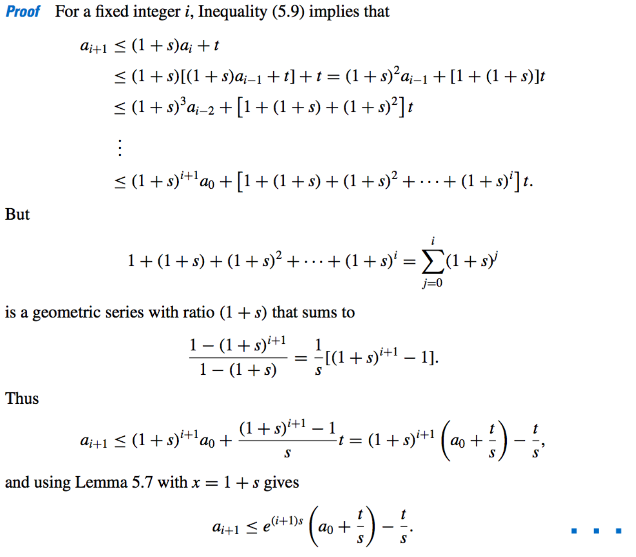
Lemma 1:

-
Lemma 2:
-
-
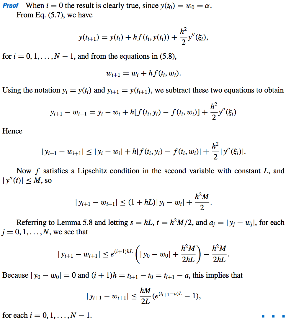
Error Bound:
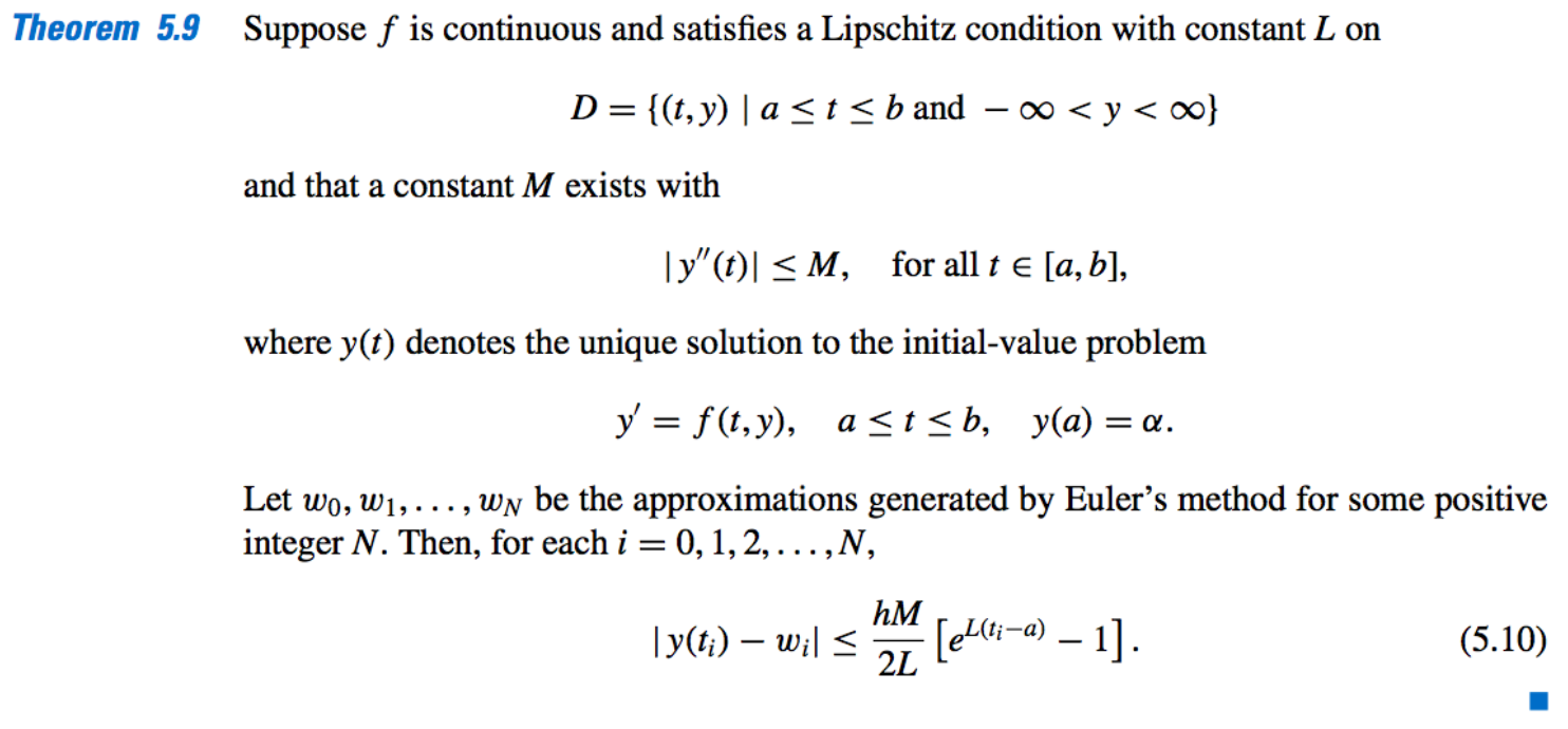
- Properties of the Error Bound Theorem:
- The Weakness of Theorem 5.9 lies in the requirement that a bound be known for the second derivative of the solution.
- However, if \(\dfrac{\partial f}{\partial t}\) and \(\dfrac{\partial f}{\partial y}\) both exist, the chain rule for partial differentiation implies that
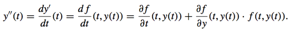
So it is at times possible to obtain an error bound for \(y''(t)\) without explicitly knowing \(y(t)\). - The Principal Importance of the error-bound formula given in Theorem 5.9 is that the bound depends linearly on the step size h.
- Consequently, diminishing the step size should give correspondingly greater accuracy to the approximations.
Finite Digit Approximations
- Euler Method [Finite-Digit Approximations]:

Where \(\delta_i\) denotes the round-off error associated with \(u_i\).
-
Error Bound for fin-dig approx. to \(y_i\) given by Euler’s method:
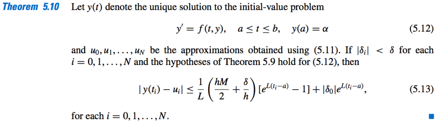
- Properties of the Error Bound on Finit-digit Approximations:
- The error bound (5.13) is no longer linear in h.
- In fact, since
\(\ \ \ \ \ \ \ \ \ \ \ \ \ \ \ \ \ \ \ \ \\) \(\lim_{h\to 0} \ (\dfrac{hM}{2} + \dfrac{\delta}{h}) = \infty,\)
the error would be expected to become large for sufficiently small values of h. - Calculus can be used to determine a lower bound for the step size h:
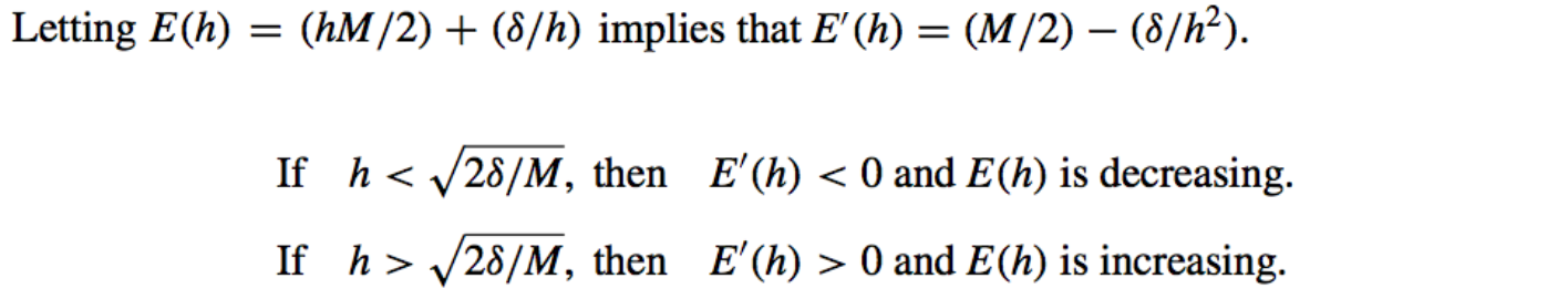
-
- The Minimal value of \(E(h)\) occurs when,
- \[h = \sqrt{\dfrac{2\delta}{M}} \ \ \ \ \ \ \ \ \ \ \ \ \ \ \ \ \ \ \ \ \ \ \ \ \ \ \ \ \ \ \ \ \ \ \ \ \ \ \ \ \ \ (5.14)\]
- Decreasing h beyond this value tends to increase the total error in the approximation; however, normally, \(\delta\) is so small that the lower bound for h doesn’t affect Euler’s Method.