• Outline of Machine Learning - Wikipedia!

Machine Learning Basics

1. Introduction and Definitions:
   • Two Approaches to Statistics:
     • Frequentest Estimators
     • Bayesian Inference
   • The Design Matrix:
     A common way for describing a dataset where it is a matrix containing a different example in each row. Each column of the matrix corresponds to a different feature.
     
2. Learning Algorithms:
   • Learning:
     A computer program is said to learn from experience \(E\) with respect to some class of tasks \(T\) and performance measure \(P\), if its performance at tasks in \(T\), as measured by \(P\), improves with experience \(E\).
   • The Task \(T\):
     Show List
   • The Performance Measure \(P\):
     A quantitative measure of the performance of a machine learning algorithm.
     We often use accuracy or error rate.
     
     
3. Machine Learning Methods:
   • List of Machine Learning Methods

     
     

4. Learning vs Optimization:
   Generalization: is the ability to perform well on previously unobserved inputs.
   Generalization (Test) Error: is defined as the expected value of the error on a new input.

   Learning vs Optimization:

   • The problem of Reducing the training error on the training set is one of optimization.
   • The problem of Reducing the training error, as well as, the generalization (test) error is one of learning.
     
     

5. Statistical Learning Theory:
   It is a framework that, under certain assumptions, allows us to study the question of “ How can we affect performance on the test set when we can observe only the training set?”

   Assumptions:

   • The training and test data are generated by a probability distribution over datasets called the data-generating process.
   • The i.i.d. assumptions:
     • The examples in each dataset are independent from each other
     • The training set and test set are identically distributed (drawn from the same probability distribution as each other)

     This assumption enables us to describe the data-generating process with a probability distribution over a single example. The same distribution is then used to generate every train example and every test example.

   • We call that shared underlying distribution the data-generating distribution, denoted \(p_{\text{data}}\)

   This probabilistic framework and the i.i.d. assumptions enable us to mathematically study the relationship between training error and test error.

6. Capacity, Overfitting, and Underfitting:
   The ML process:
   We sample the training set, then use it to choose the parameters to reduce training set error, then sample the test set.
   Under this process, the expected test error is greater than or equal to the expected value of training error.

   The factors determining how well a machine learning algorithm will perform are its ability to:

   1. Make the training error small
   2. Make the gap between training and test error small

   These two factors correspond to the two central challenges in machine learning: underfitting and overfitting.
   Underfitting: occurs when the model is not able to obtain a sufficiently low error value on the training set.
   Overfitting: occurs when the gap between the training error and test error is too large.

   We can control whether a model is more likely to overfit or underfit by altering its capacity.
   Capacity: a models capacity is its ability to fit a wide variety of functions.

   • Models with low capacity may struggle to fit the training set.
   • Models with high capacity can overfit by memorizing properties of the training set that do not serve them well on the test set.

   One way to control the capacity of a learning algorithm is by choosing its hypothesis space.
   Hypothesis Space: the set of functions that the learning algorithm is allowed to select as being the solution.

   Statistical learning theory provides various means of quantifying model capacity.Among these, the most well known is the Vapnik-Chervonenkis (VC) dimension.
   The VC Dimension: is defined as being the largest possible value of \(m\) for which there exists a training set of \(m\) different \(\mathbf{x}\) points that the classifier can label arbitrarily.
   It measure the capacity of a binary classifier.

   Quantifying the capacity of the model enables statistical learning theory to make quantitative predictions. The most important results in statistical learning theory show that the discrepancy between training error and generalization error is bounded from above by a quantity that grows as the model capacity grows but shrinks as the number of training examples increases.

   

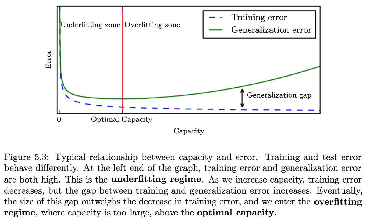
   Effective capacity and Representational Capacity…

7. Regularization:
   Regularization is a (more general) way of controlling a models capacity by allowing us to express preference for one function over another in the same hypothesis space; instead of including or excluding members from the hypothesis space completely.

   We can think of excluding a function from a hypothesis space as expressing an infinitely strong preference against that function.

   Regularization can be defined as any modification we make to a learning algorithm that is intended to reduce its generalization error but not its training error.

   Example: Weight Decay
   It is a regularization form that adds the \(L^2\) norm of the weights to the cost function; allowing us to express preference for smaller weights. It is controlled by a hyperparameter \(\lambda\).

   $$J(\boldsymbol{w})=\mathrm{MSE}_ {\mathrm{train}}+\lambda \boldsymbol{w}^{\top} \boldsymbol{w}$$

   This gives us solutions that have a smaller slope, or that put weight on fewer of the features.

   More generally, the regularizer penalty of weight decay is:

   $$\Omega(\boldsymbol{w})=\boldsymbol{w}^{\top} \boldsymbol{w}$$

   
   

8. Point Estimation:
   Point estimation is the attempt to provide the single “best” prediction of some quantity of interest. In general the quantity of interest can be a single parameter or a vector of parameters in some parametric model, such as the weights in linear regression, but it can also be a whole function.
   
   

9. Estimators:
   A Point Estimator or statistic is any function of the data:

   $$\hat{\boldsymbol{\theta}}_{m}=g\left(\boldsymbol{x}^{(1)}, \ldots, \boldsymbol{x}^{(m)}\right)$$

   such that a good estimator is a function whose output is close to the true underlying \(\theta\) that generated the training data.

   We assume that the true \(\boldsymbol{\theta}\) is fixed, and that \(\hat{\boldsymbol{\theta}}\) is a function of the data, which is drawn from a random process, making \(\hat{\boldsymbol{\theta}}\) a random variable.
   Thus, a point estimator is a random variable.

   Function Estimation/Approximation refers to estimation of the relationship between input and target data.
   I.E. We are trying to predict a variable \(y\) given an input vector \(x\), and we assume that there is a function \(f(x)\) that describes the approximate relationship between \(y\) and \(x\).
   If we assume that: \(y = f(x) + \epsilon\), where \(\epsilon\) is the part of \(y\) that is not predictable from \(x\); then we are interested in approximating \(f\) with a model or estimate \(\hat{f}\).

   Function estimation is really just the same as estimating a parameter \(\boldsymbol{\theta}\); the function estimator \(\hat{f}\) is simply a point estimator in function space.

   Linear Regression and Polynomial Regression both illustrate scenarios that may be interpreted as either estimating a parameter \(\boldsymbol{w}\) or estimating a function \(f\) mapping from \(\boldsymbol{x}\) to \(y\).

   • Estimators as statistics and their probability distributions
   • Estimators in ML
   • Plain and Simple Estimators (TF)

   Notes:

   • weights \(\boldsymbol{w}\) == parameters \(\theta\)
   • parameter/point estimation == function estimation
     Linear Regression and Polynomial Regression both illustrate scenarios that may be interpreted as either estimating a parameter \(\boldsymbol{w}\) or estimating a function \(f\) mapping from \(\boldsymbol{x}\) to \(y\).
   • we can use the theory and tools for analyzing point estimators and apply them to function estimators (e.g. bias/var decomp etc.)

   
   

10. Properties of Estimators - Bias and Variance:
    The Bias of an estimator is:

    $$ \operatorname{bias}\left(\hat{\boldsymbol{\theta}}_{m}\right)=\mathbb{E}\left(\hat{\boldsymbol{\theta}}_{m}\right)-\boldsymbol{\theta} $$

    where the expectation is over the data (seen as samples from a random variable) and \(\theta\) is the true underlying value of \(\theta\) used to define the data-generating distribution.

    • Unbiased Estimators: An estimator \(\hat{\boldsymbol{\theta}}_{m}\) is said to be unbiased if \(\operatorname{bias}\left(\hat{\boldsymbol{\theta}}_{m}\right)=\mathbf{0}\), which implies that \(\mathbb{E}\left(\hat{\boldsymbol{\theta}}_{m}\right)=\boldsymbol{\theta}\).
    • Asymptotically Unbiased Estimators: An estimator is said to be asymptotically unbiased if \(\lim _{m \rightarrow \infty} \operatorname{bias}\left(\hat{\boldsymbol{\theta}}_{m}\right)=\mathbf{0},\) which implies that \(\lim _{m \rightarrow \infty} \mathbb{E}\left(\hat{\boldsymbol{\theta}}_{m}\right)=\boldsymbol{\theta}\)

    The Variance of an estimator is a way to measure how much we expect the estimator to vary as a function of the data sample, defined, simply, as the variance over the training set random variable \(\hat{\theta}\):

    $$ \operatorname{Var}(\hat{\theta}) $$

    The Standard Error \(\operatorname{SE}(\hat{\theta})\), of an estimator, is the square root of the variance.

    • E.g. The Standard Error of the (Sample) Mean:
      \(\operatorname{SE}\left(\hat{\mu}_{m}\right)=\sqrt{\operatorname{Var}\left[\frac{1}{m} \sum_{i=1}^{m} x^{(i)}\right]}=\frac{\sigma}{\sqrt{m}}\)
      Where \(\sigma^2\) is the true variance of the samples \(x^i\).

      Derivation

    Unfortunately, neither the square root of the sample variance nor the square root of the unbiased estimator of the variance provide an unbiased estimate of the standard deviation.

    • Properties of the Sample Mean Estimator (Derivations)
      
      
11. Generalization Error from Standard Error (of the mean):
    We often estimate the generalization error by computing the sample mean of the error on the test set.
    Taking advantage of the central limit theorem, which tells us that the mean will be approximately distributed with a normal distribution, we can use the standard error to compute the probability that the true expectation falls in any chosen interval.
    For example, the \(95\%\) confidence interval centered on the mean \(\hat{\mu}_ {m}\) is:

    $$\left(\hat{\mu}_{m}-1.96 \mathrm{SE}\left(\hat{\mu}_{m}\right), \hat{\mu}_{m}+1.96 \mathrm{SE}\left(\hat{\mu}_{m}\right)\right)$$

    under the normal distribution with mean \(\hat{\mu}_{m}\) and variance \(\mathrm{SE}\left(\hat{\mu}_{m}\right)^{2}\).

    We say that algorithm \(\boldsymbol{A}\) is better than algorithm \(\boldsymbol{B}\) if the <upper bound of the \(95\%\) confidence interval for the error of algorithm \(\boldsymbol{A}\)> is less than the <lower bound of the \(95\%\) confidence interval for the error of algorithm \(\boldsymbol{B}\)>.

12. The Bias Variance Trade-off:
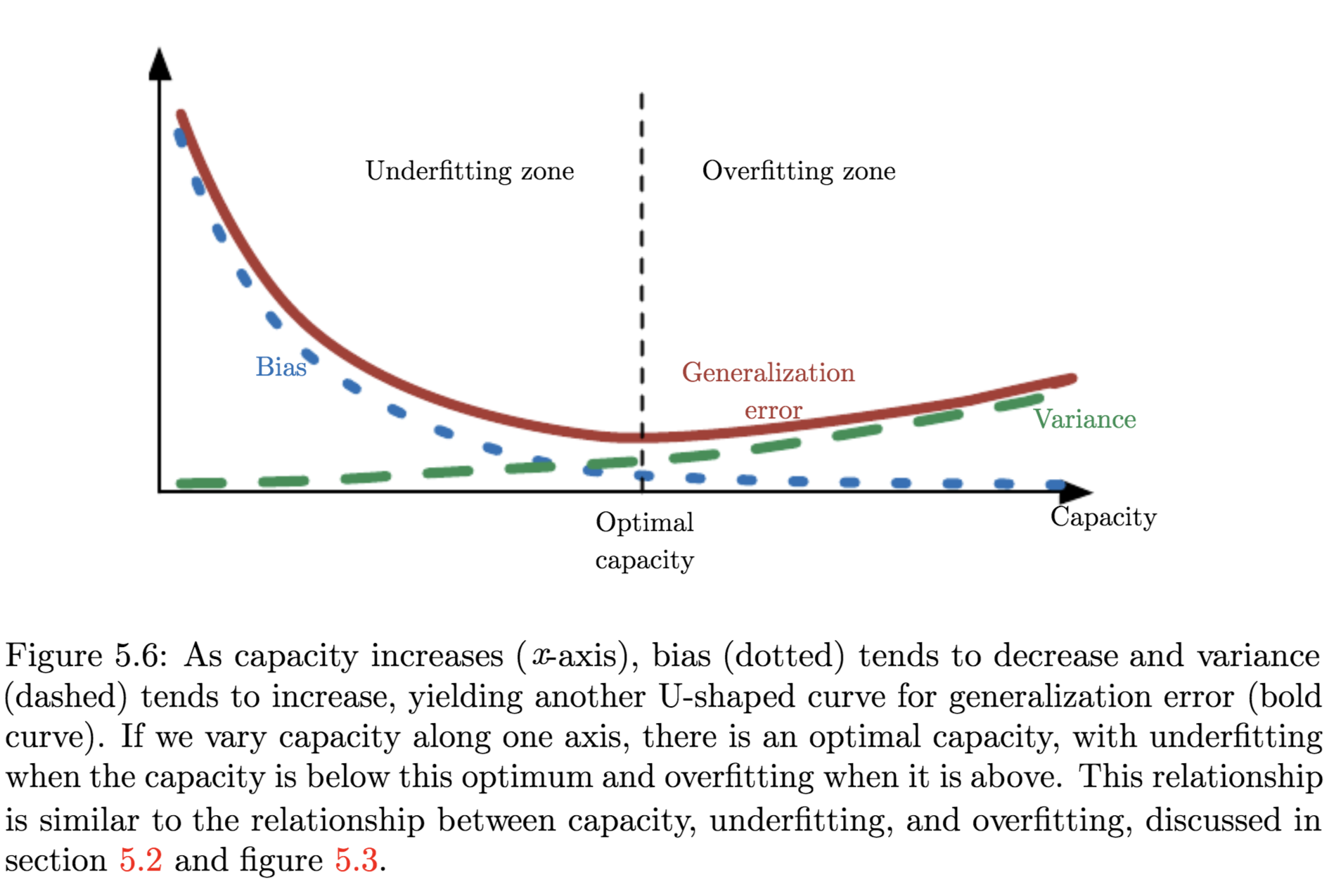
    Bias and variance measure two different sources of error in an estimator:
    • Bias: measures the expected deviation from the true value of the function or parameter
    • Variance: provides a measure of the deviation from the expected estimator value that any particular sampling of the data is likely to cause

    Evaluating Models - Trading off Bias and Variance:

    • The most common way to negotiate this trade-off is to use cross-validation
    • Alternatively, we can also compare the mean squared error (MSE) of the estimates:

      $$\begin{aligned} \mathrm{MSE} &=\mathbb{E}\left[\left(\hat{\theta}_{m}-\theta\right)^{2}\right] \\ &=\operatorname{Bias}\left(\hat{\theta}_{m}\right)^{2}+\operatorname{Var}\left(\hat{\theta}_{m}\right) \end{aligned}$$

      The MSE measures the overall expected deviation — in a squared error sense — between the estimator and the true value of the parameter \(\theta\).

    Capacity and Bias/Variance

13. Properties of Estimators - Consistency:
    Consistency is a property implying that as the number of data points \(m\) in our dataset increases, our point estimates converge to the true value of the corresponding parameters. Formally:

    $$\mathrm{plim}_{m \rightarrow \infty} \hat{\theta}_{m}=\theta$$

    Where:
    \({\text { The symbol plim indicates convergence in probability, meaning that for any } \epsilon>0,}\)

    $${P\left(\vert\hat{\theta}_ {m}-\theta \vert>\epsilon\right) \rightarrow 0 \text { as } m \rightarrow \infty}$$

    Sometimes referred to as Weak Consistency

    Strong Consistency applies to almost sure convergence of \(\hat{\theta}\) to \(\theta\).

    Consistency and Asymptotic Bias:

    • Consistency ensures that the bias induced by the estimator diminishes as the number of data examples grows.
    • However, asymptotic unbiasedness does not imply consistency
      • It is also useful to note that by Chebyshev’s inequality, if the variance tends to zero then asymptotic unbiasedness implies consistency stex.

    Consistency implies both unbiasedness and low variance and therefore, unbiasedness alone is not sufficient to imply consistency.

    
    

14. Maximum Likelihood Estimation (MLE):
    MLE is a method/principle from which we can derive specific functions that are good estimators for different models.

    Likelihood is the probability of the data given the parameters of the model

    Let \(\mathbb{X}=\left\{\boldsymbol{x}^{(1)}, \ldots, \boldsymbol{x}^{(m)}\right\}\) be a set of \(m\) examples drawn independently from the true but unknown data-generating distribution \(p_{\text{data}}(\mathbf{x})\), and let \(p_{\text{model}}(\mathbf{x} ; \boldsymbol{\theta})\) be a parametric family of probability distributions over the same space indexed by \(\boldsymbol{\theta}\)¹,
    The Maximum Likelihood Estimator for \(\boldsymbol{\theta}\) is:

    $$\begin{aligned} \boldsymbol{\theta}_{\mathrm{ML}} &=\underset{\boldsymbol{\theta}}{\arg \max } \: p_{\text{model}}(\mathbb{X} ; \boldsymbol{\theta}) \\ &=\underset{\boldsymbol{\theta}}{\arg \max } \prod_{i=1}^{m} p_{\text{model}}\left(\boldsymbol{x}^{(i)} ; \boldsymbol{\theta}\right) \end{aligned}$$

    We take the \(log\) for numerical stability:

    $$\boldsymbol{\theta}_{\mathrm{ML}}=\underset{\boldsymbol{\theta}}{\arg \max } \sum_{i=1}^{m} \log p_{\text{model}}\left(\boldsymbol{x}^{(i)} ; \boldsymbol{\theta}\right) \tag{5.58}$$

    Because the \(\text { arg max }\) does not change when we rescale the cost function, we can divide by \(m\) to obtain a version of the criterion that is expressed as an expectation with respect to the empirical distribution \(\hat{p}_ {\text{data}}\) defined by the training data:

    $$\boldsymbol{\theta}_{\mathrm{ML}}=\underset{\boldsymbol{\theta}}{\arg \max } \: \underset{\mathbf{x} \sim \hat{p}_\text{data}}{\mathbb{E}} [\log p_{\text{model}}(\boldsymbol{x} ; \boldsymbol{\theta})] \tag{5.59}$$

    MLE as Minimizing KL-Divergence between the Empirical dist. and the model dist.:
    We can interpret maximum likelihood estimation as minimizing the dissimilarity between the empirical distribution \(\hat{p}_ {\text{data}}\), defined by the training set, and the model distribution, with the degree of dissimilarity between the two measured by the KL divergence.

    • The KL-divergence is given by:

      $$D_{\mathrm{KL}}\left(\hat{p}_{\text{data}} \| p_{\text{model}}\right)=\mathbb{E}_{\mathbf{x} \sim \hat{p}_{\text{data}}}\left[\log \hat{p}_{\text{data}}(\boldsymbol{x})-\log p_{\text{model}}(\boldsymbol{x})\right] \tag{5.60}$$

      The term on the left is a function only of the data-generating process, not the model. This means when we train the model to minimize the KL divergence, we need only minimize:

    $$-\mathbb{E}_{\mathbf{x} \sim \hat{p}_{\text{data}}}\left[\log p_{\text{model}}(\boldsymbol{x})\right] \tag{5.61}$$

    which is of course the same as the maximization in equation \(5.59\).

    Minimizing this KL-divergence corresponds exactly to minimizing the cross-entropy between the distributions.

    Any loss consisting of a negative log-likelihood is a cross-entropy between the empirical distribution defined by the training set and theprobability distribution defined by model.
    E.g. MSE is the cross-entropy between the empirical distribution and a Gaussian model.

    We can thus see maximum likelihood as an attempt to make the model distribution match the empirical distribution \(\hat{p} _ {\text{data}}\)².

    Maximum likelihood thus becomes minimization of the negative log-likelihood(NLL), or equivalently, minimization of the cross-entropy³.

    • MLE as Minimizing KL-div

    Conditional Log-Likelihood (MLE for Supervised Learning):
    The maximum likelihood estimator can readily be generalized to estimate a conditional probability \(P(\mathbf{y} | \mathbf{x} ; \boldsymbol{\theta})\) in order to predict \(\mathbf{y}\) given \(\mathbf{x}\). If \(X\) represents all our inputs and \(Y\) all our observed targets, then the conditional maximum likelihood estimator is:

    $$\boldsymbol{\theta}_ {\mathrm{ML}}=\underset{\boldsymbol{\theta}}{\arg \max } \: P(\boldsymbol{Y} | \boldsymbol{X} ; \boldsymbol{\theta}) \tag{5.62}$$

    and the log-likelihood estimator is:

    $$\boldsymbol{\theta}_{\mathrm{ML}}=\underset{\boldsymbol{\theta}}{\arg \max } \sum_{i=1}^{m} \log P\left(\boldsymbol{y}^{(i)} | \boldsymbol{x}^{(i)} ; \boldsymbol{\theta}\right) \tag{5.63}$$

    Properties of Maximum Likelihood Estimator:
    The main appeal of the maximum likelihood estimator is that it can be shown to be the best estimator asymptotically, as the number of examples \(m \rightarrow \infty\), in terms of its rate of convergence as \(m\) increases.

    • Consistency: as the number of training examples approaches infinity, the maximum likelihood estimate of a parameter converges to the true value of the parameter, under the following conditions:
      • The true distribution \(p_{\text{data}}\) must lie within the model family \(p_{\text{model}}(\cdot ; \boldsymbol{\theta})\). Otherwise, no estimator can recover \(p_{\text{data}}\).
      • The true distribution \(p_{\text{data}}\) must correspond to exactly one value of \(\boldsymbol{\theta}\). Otherwise, maximum likelihood can recover the correct \(p_{\text{data}}\) but will not be able to determine which value of \(\boldsymbol{\theta}\) was used by the data-generating process.
    • Statistical Efficiency: meaning that one consistent estimator may obtain lower generalization error for a fixed number of samples \(m\), or equivalently, may require fewer examples to obtain a fixed level of generalization error.⁴
      The Cramér-Rao lower bound shows that no consistent estimator has a lower MSE than the maximum likelihood estimator.
      
      
15. Maximum A Posteriori (MAP) Estimation:
    The MAP estimate chooses the point of maximal posterior probability by allowing the prior to influence the choice of the point estimate:

    $$\boldsymbol{\theta}_ {\mathrm{MAP}}=\underset{\boldsymbol{\theta}}{\arg \max } p(\boldsymbol{\theta} | \boldsymbol{x})=\underset{\boldsymbol{\theta}}{\arg \max } \log p(\boldsymbol{x} | \boldsymbol{\theta})+\log p(\boldsymbol{\theta}) \tag{5.79}$$

    Many regularized estimation strategies, such as maximum likelihood learning regularized with weight decay, can be interpreted as making the MAP approximation to Bayesian inference.

    E.g. MAP Bayesian inference with a Gaussian prior on the weights corresponds to weight decay Regularization:
    consider a linear regression model with a Gaussian prior on the weights \(\mathbf{w}\). If this prior is given by \(\mathcal{N}\left(\boldsymbol{w} ; \mathbf{0}, \frac{1}{\lambda} \boldsymbol{I}^{2}\right)\), then the log-prior term in equation \(5.79\) is proportional to the familiar \(\lambda w^{T} w\) weight decay penalty, plus a constant.

    This view applies when the regularization consists of adding an extra term to the objective function that corresponds to \(\log p(\boldsymbol{\theta})\) (i.e. logarithm of a probability distribution).

The Mathematics of Neural Networks

1. Derivative:
   The derivative of a function is the amount that the value of a function changes when the input changes by an \(\epsilon\) amount:

   $$f'(a)=\lim_{h\to 0}{\frac {f(a+h)-f(a)}{h}}. \\ \text{i.e. } f(x + \epsilon)\approx f(x)+\epsilon f'(x) $$

   The Chain Rule is a way to compute the derivative of composite functions.
   If \(y = f(x)\) and \(z = g(y)\):

   $$\dfrac{\partial z}{\partial x} = \dfrac{\partial z}{\partial y} \dfrac{\partial y}{\partial x}$$

2. Gradient: (Vector in, Scalar out)
   Gradients generalize derivatives to scalar functions of several variables
   

   Property: the gradient of a function \(\nabla f(x)\) points in the direction of steepest ascent from \(x\).
   
   

3. The Jacobian: (Vector in, Vector out)

   The Jacobian of \(f: \mathbb{R}^n \rightarrow \mathbb{R}^m\) is a matrix of first-order partial derivatives of a vector-valued function:

   

   The Chain Rule:
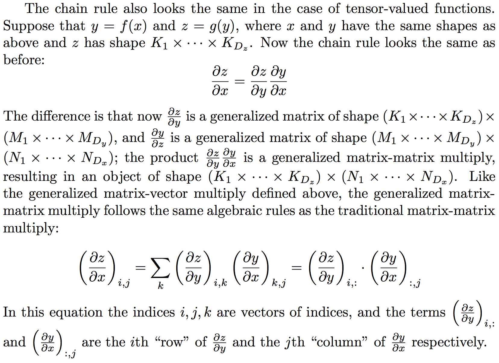
   Let \(f : \mathbb{R}^N \rightarrow \mathbb{R}^M\) and \(g : \mathbb{R}^M \rightarrow \mathbb{R}^ K\); and let \(x \in \mathbb{R}^N, y \in \mathbb{R}^M\), and \(z \in \mathbb{R}^K\) with \(y = f(x)\) and \(z = g(y)\):

   \[\dfrac{\partial z}{\partial x} = \dfrac{\partial z}{\partial y} \dfrac{\partial y}{\partial x}\]

   where, \(\dfrac{\partial z}{\partial y} \in \mathbb{R}^{K \times M}\) matrix, \(\dfrac{\partial y}{\partial x} \in \mathbb{R}^{M \times N}\) matrix, and \(\dfrac{\partial z}{\partial x} \in \mathbb{R}^{K \times N}\) matrix;
   the multiplication of \(\dfrac{\partial z}{\partial y}\) and \(\dfrac{\partial y}{\partial x}\) is a matrix multiplication.

4. The Generalized Jacobian: (Tensor in, Tensor out)

   A Tensor is a D-dimensional grid of number.

   Suppose that \(f: \mathbb{R}^{N_1 \times \cdots \times N_{D_x}} \rightarrow \mathbb{R}^{M_1 \times \cdots \times M_{D_y}}\).
   If \(y = f(x)\) then the derivative \(\dfrac{\partial y}{\partial x}\) is a generalized Jacobian - an object with shape:

   \[(M_1 \times \cdots \times M_{D_y}) \times (N_1 \times \cdots \times N_{D_x})\]

   we can think of the generalized Jacobian as generalization of a matrix, where each “row” has the same shape as \(y\) and each “column” has the same shape as \(x\).

   Just like the standard Jacobian, the generalized Jacobian tells us the relative rates of change between all elements of \(x\) and all elements of \(y\):

   \[(\dfrac{\partial y}{\partial x})_{i,j} = \dfrac{\partial y_i}{\partial x_j} \in \mathbb{R}\]

   Just as the derivative, the generalized Jacobian gives us the relative change in \(y\) given a small change in \(x\):

   \[f(x + \delta x)\approx f(x)+ f'(x) \delta x = y + \dfrac{\partial y}{\partial x}\delta x\]

   where now, \(\delta x\) is a tensor in \(\mathbb{R}{N_1 \cdots N_{d_x}}\) and \(\dfrac{\partial y}{\partial x}\) is a generalized matrix in \(\mathbb{R}^{(M_1 \times \cdots \times M_{D_y}) \times (N_1 \times \cdots \times N_{D_x})}\).
   The product \(\dfrac{\partial y_i}{\partial x_j} \delta x\) is, therefore, a generalized matrix-vector multiply, which results in a tensor in \(\mathbb{R}^{M_1 \times \cdots \times M_{D_y}}\).

   The generalized matrix-vector multiply follows the same algebraic rules as a traditional matrix-vector multiply:

   

   

   The Chain Rule:

   

5. The Hessian:

   The Hessian Matrix of a scalar function \(f: \mathbb{R}^d \rightarrow \mathbb{R}\) is a matric of second-order partial derivatives:

   

   Properties:

   • The Hessian matrix is symmetric - since we usually work with smooth/differentiable functions - due to Clairauts Theorem.

     Clairauts Theorem: if the partial derivatives are continuous, the order of differentiation can be interchanged

   • The Hessian is used in some optimization algorithms such as Newton’s method
   • It is expensive to calculate but can drastically reduce the number of iterations needed to converge to a local minimum by providing information about the curvature of \(f\)

6. Matrix Calculus:

   Important Identities:

   \[{\frac {\partial {\mathbf {a}}^{\top }{\mathbf {x}}}{\partial {\mathbf {x}}}}={\frac {\partial {\mathbf {x}}^{\top }{\mathbf {a}}}{\partial {\mathbf {x}}}}= a \\ {\frac {\partial {\mathbf {x}}^{\top }{\mathbf {A}}{\mathbf {x}}}{\partial {\mathbf {x}}}}= ({\mathbf {A}}+{\mathbf {A}}^{\top }){\mathbf {x}} \\ {\frac {\partial {\mathbf {x}}^{\top }{\mathbf {A}}{\mathbf {x}}}{\partial {\mathbf {x}}}}= 2{\mathbf {A}}{\mathbf {x}} \:\:\:\:\: \text{[Symmetric } A\text{]}\]

   Identities

   The Product Rule:

   \[{\displaystyle {\begin{aligned}\nabla (\mathbf {A} \cdot \mathbf {B} )&=(\mathbf {A} \cdot \nabla )\mathbf {B} +(\mathbf {B} \cdot \nabla )\mathbf {A} +\mathbf {A} \times (\nabla \times \mathbf {B} )+\mathbf {B} \times (\nabla \times \mathbf {A} )\\&=\mathbf {J} _{\mathbf {A} }^{\mathrm {T} }\mathbf {B} +\mathbf {J}_{\mathbf {B} }^{\mathrm {T} }\mathbf {A} \\&=\nabla \mathbf {A} \cdot \mathbf {B} +\nabla \mathbf {B} \cdot \mathbf {A} \ \end{aligned}}}\\ \implies \\ \nabla (fg) = (f')^T g + (g')^T f\]

   Thus, we set our function \(h(x) = \langle f(x), g(x) \rangle = f(x)^T g(x)\); then,

   \[\nabla h(x) = f'(x)^T g(x) + g'(x)^T f(x).\]

The answer to the product rule is as follows:

\(\nabla (f^Tg) = f'g + g'f\)
or

\[\nabla (x^TAx) = \nabla (x)^T(Ax) = (x)'(Ax) + (Ax)'x = Ax + A^Tx = (A+A^T)x\]

Challenges in Machine Learning

1. The Curse of Dimensionality:
   It is a phenomena where many machine learning problems become exceedingly difficult when the number of dimensions in the data is high.

   • The number of possible distinct configurations of a set of variables increases exponentially as the number of variables increases:
     Capacity and Bias/Variance
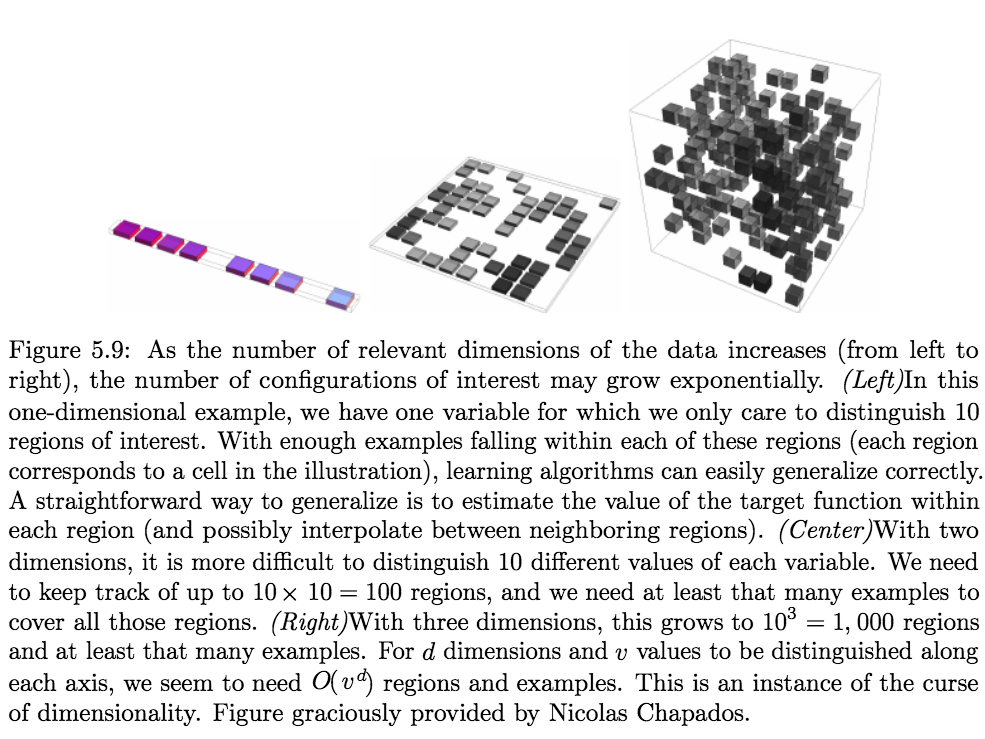
     • Statistical Challenge: the number of possible configurations of \(x\) is much larger than the number of training examples
   • Further Reading (Concepts)
   • Yoshua Bengio on Curse of Dimensionality (Quora)
     
     
2. Local Constancy and Smoothness Regularization:
   Prior believes about the particular data-set/learning-problem can be incorporated as:
   • Beliefs about the distribution of parameters
   • Beliefs about the properties of the estimating function
     Expressed implicitly by choosing algorithms that are biased toward choosing some class of functions over another, even though these biases may not be expressed (or even be possible to express) in terms of a probability distribution representing our degree of belief in various functions.

   The Local Constancy (Smoothness) Prior: states that the function we learn should not change very much within a small region.
   Mathematically, traditional ML methods are designed to encourage the learning process to learn a function \(f^\ast\) that satisfies the condition:
   \(\:\:\:\:\:\:\:\) \(\:\:\:\:\:\:\:\) \(f^{*}(\boldsymbol{x}) \approx f^{*}(\boldsymbol{x}+\epsilon)\)
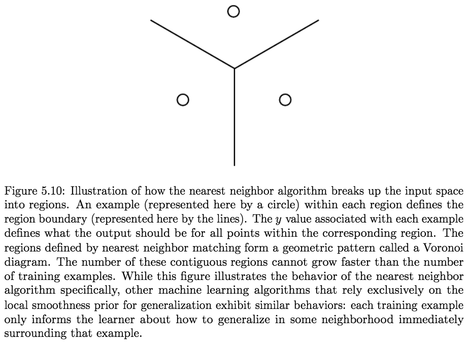
   for most configurations \(x\) and small change \(\epsilon\).

   • Example: K-Means

   A Local Kernel can be thought of as a similarity function that performs template matching, by measuring how closely a test example \(x\) resembles each training example \(x^{(i)}\).
   Much of the modern motivation for Deep Learning is derived from studying the limitations of local template matching and how deep models are able to succeed in cases where local template matching fails (Bengio et al., 2006b).

   • The Curse of Dimensionality for Local Kernel Machines (paper!)

   Example: Decision Trees

   In general, to distinguish \(\mathcal{O}(k)\) regions in input space, all these methods require \(\mathcal{O}(k)\) examples. Typically there are \(\mathcal{O}(k)\) parameters, with \(\mathcal{O}(1)\) parameters associated with each of the \(\mathcal{O}(k)\) regions.

   Key Takeaways:

   • Is there a way to represent a complex function that has many more regions to be distinguished than the number of training examples?
     Clearly, assuming only smoothness of the underlying function will not allow a learner to do that.
     The smoothness assumption and the associated nonparametric learning algorithms work extremely well as long as there are enough examples for the learning algorithm to observe high points on most peaks and low points on most valleys of the true underlying function to be learned.
   • Is it possible to represent a complicated function efficiently? and if it is complicated, Is it possible for the estimated function to generalize well to new inputs?
     Yes.
     The key insight is that a very large number of regions, such as \(\mathcal{O}(2^k)\), can be defined with \(\mathcal{O}(k)\) examples, so long as we introduce some dependencies between the regions through additional assumptions about the underlying data-generating distribution.
     In this way, we can actually generalize non-locally (Bengio and Monperrus, 2005; Bengio et al., 2006c).
     Many different deep learning algorithms provide implicit or explicit assumptions that are reasonable for a broad range of AI tasks in order to capture these advantages.
     • Non-Local Generalization (for an Algorithm)
     • Non-Local VS Local Generalization correspond to Distributed VS Local Representations
   • Deep Learning VS Machine Learning:
     The core idea in deep learning is that we assume that the data was generated by the composition of factors, or features, potentially at multiple levels in a hierarchy.
     These apparently mild assumptions allow an exponential gain in the relationship between the number of examples and the number of regions that can be distinguished.
     The exponential advantages conferred by the use of deep distributed representations counter the exponential challenges posed by the curse of dimensionality.
     (Many other similarly generic assumptions can further improve deep learning algorithms).
     • Further Reading: (on the exponential gain) Sections: 6.4.1, 15.4 and 15.5.
     • Why generic assumptions not specific assumptions!

3. Manifold Learning:
   A Manifold - a connected region - is a set of points associated with a neighborhood around each point. From any given point, the manifold locally appears to be a Euclidean space.
   

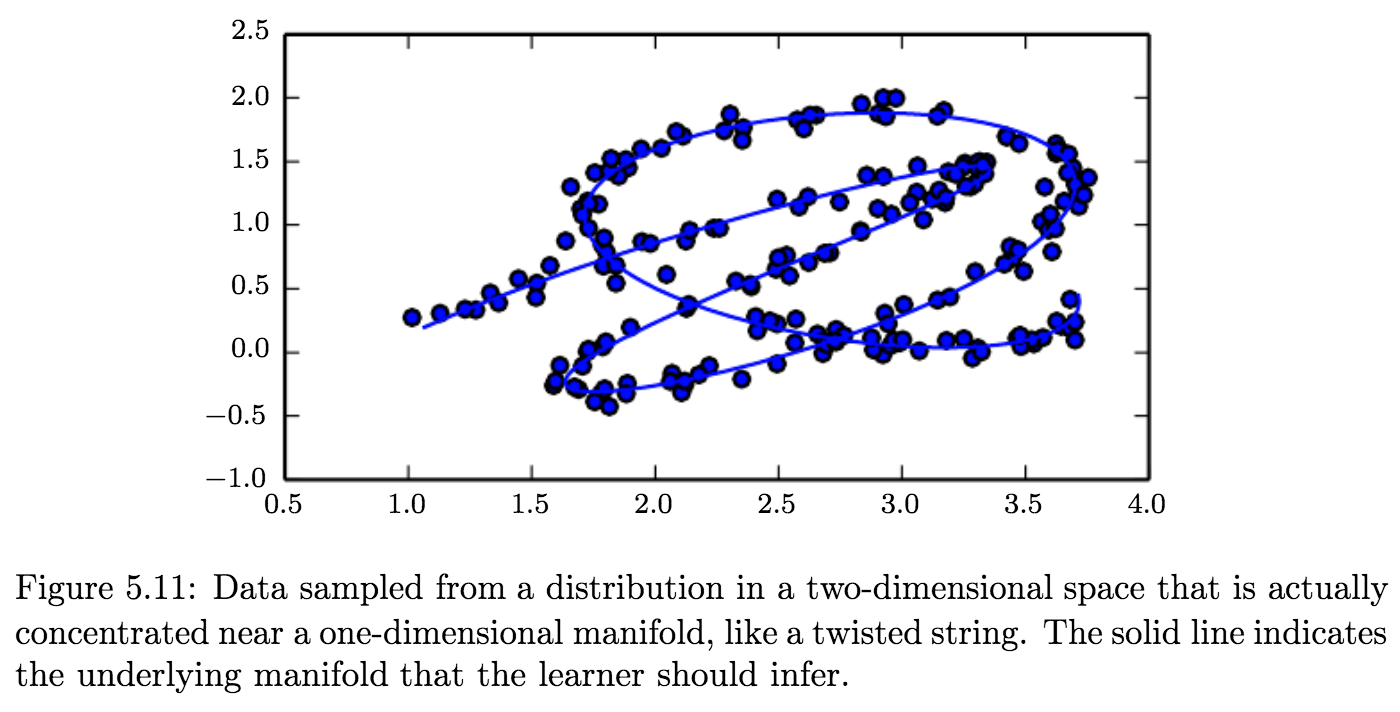
   Manifolds in ML:
   In ML, the term is used loosely to designate a connected set of points that can be approximated well by considering only a small number of degrees of freedom, or dimensions, embedded in a higher-dimensional space. Each dimension corresponds to a local direction of variation.
   In the context of machine learning, we allow the dimensionality of the manifold to vary from one point to another. This often happens when a manifold intersects itself. For example, a figure eight is a manifold that has a single dimension in most places but two dimensions at the intersection at the center.
   Manifold Assumptions:
   Discussion
   We assume that the data lies along a low-dimensional manifold:

   • May not always be correct or useful
   • In the context of AI tasks (e.g. processing images, sounds, or text): At least approximately correct.
     To show that is true we need to argue two points:
     • The probability distribution over images, text strings, and sounds that occur in real life is highly concentrated.
       Example/proof: The Manifold of Natural Images

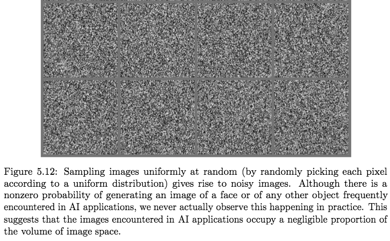
       Uniform noise essentially never resembles structured inputs from these domains.

     • We must, also, establish that the examples we encounter are connected to each other by other examples, with each example surrounded by other highly similar examples that can be reached by applying transformations to traverse the manifold:
       Informally, we can imagine such neighborhoods and transformations:
       In the case of images, we can think of many possible transformations that allow us to trace out a manifold in image space: we can gradually dim or brighten the lights, gradually move or rotate objects in the image, gradually alter the colors on the surfaces of objects, and so forth.

       Multiple manifolds are likely involved in most applications. For example,the manifold of human face images may not be connected to the manifold of cat face images.
       Rigorous Results: (Cayton, 2005; Narayanan and Mitter,2010; Schölkopf et al., 1998; Roweis and Saul, 2000; Tenenbaum et al., 2000; Brand,2003; Belkin and Niyogi, 2003; Donoho and Grimes, 2003; Weinberger and Saul,2004)

   Benefits:
   When the data lies on a low-dimensional manifold, it can be most natural for machine learning algorithms to represent the data in terms of coordinates on the manifold, rather than in terms of coordinates in \(\mathbb{R}^n\).
   E.g. In everyday life, we can think of roads as 1-D manifolds embedded in 3-D space. We give directions to specific addresses in terms of address numbers along these 1-D roads, not in terms of coordinates in 3-D space.

   Learning Manifold Structure: figure 20.6