Table of Contents
CNNs in CV
CNNs in NLP
CNNs Architectures
Convnet Ch.9 Summary (blog)
Introduction
- CNNs:
In machine learning, a convolutional neural network (CNN, or ConvNet) is a class of deep, feed-forward artificial neural networks that has successfully been applied to analyzing visual imagery.
In general, it works on data that have grid-like topology.E.g. Time-series data (1-d grid w/ samples at regular time intervals), image data (2-d grid of pixels).
Convolutional networks are simply neural networks that use convolution in place of general matrix multiplication in at least one of their layers.
- The Big Idea:
CNNs use a variation of multilayer Perceptrons designed to require minimal preprocessing. In particular, they use the Convolution Operation.
The Convolution leverage three important ideas that can help improve a machine learning system:- Sparse Interactions/Connectivity/Weights:
Unlike FNNs, where every input unit is connected to every output unit, CNNs have sparse interactions. This is accomplished by making the kernel smaller than the input.
Benefits:- This means that we need to store fewer parameters, which both,
- Reduces the memory requirements of the model and
- Improves its statistical efficiency
- Also, Computing the output requires fewer operations
- In deep CNNs, the units in the deeper layers interact indirectly with large subsets of the input which allows modelling of complex interactions through sparse connections.
These improvements in efficiency are usually quite large.
If there are \(m\) inputs and \(n\) outputs, then matrix multiplication requires \(m \times n\) parameters, and the algorithms used in practice have \(\mathcal{O}(m \times n)\) runtime (per example). If we limit the number of connections each output may have to \(k\), then the sparsely connected approach requires only \(k \times n\) parameters and \(\mathcal{O}(k \times n)\) runtime.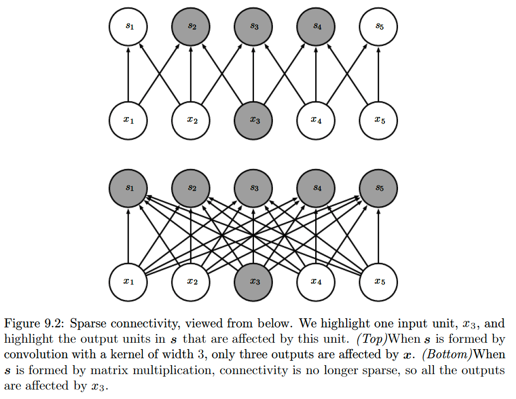
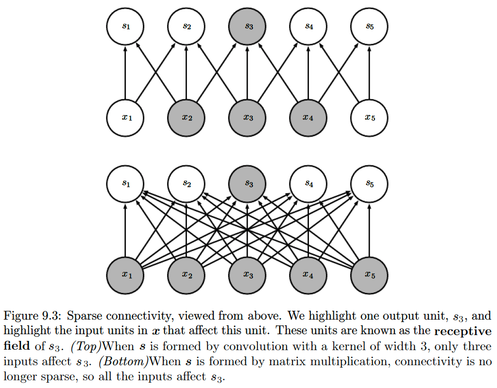
- This means that we need to store fewer parameters, which both,
-
Parameter Sharing:
refers to using the same parameter for more than one function in a model.Benefits:
- This means that rather than learning a separate set of parameters for every location, we learn only one set of parameters.
- This does not affect the runtime of forward propagation—it is still \(\mathcal{O}(k \times n)\)
- But it does further reduce the storage requirements of the model to \(k\) parameters (\(k\) is usually several orders of magnitude smaller than \(m\))
Convolution is thus dramatically more efficient than dense matrix multiplication in terms of the memory requirements and statistical efficiency.
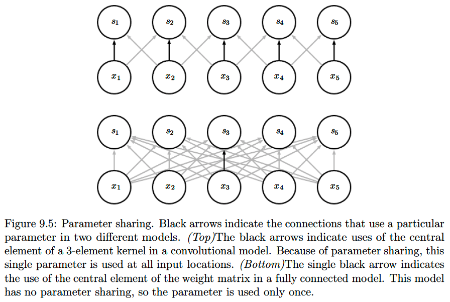
- This means that rather than learning a separate set of parameters for every location, we learn only one set of parameters.
- Equivariant Representations:
For convolutions, the particular form of parameter sharing causes the layer to have a property called equivariance to translation.A function is equivariant means that if the input changes, the output changes in the same way.
Specifically, a function \(f(x)\) is equivariant to a function \(g\) if \(f(g(x)) = g(f(x))\).Thus, if we move the object in the input, its representation will move the same amount in the output.
Benefits:
- It is most useful when we know that some function of a small number of neighboring pixels is useful when applied to multiple input locations (e.g. edge detection)
- Shifting the position of an object in the input doesn’t confuse the NN
- Robustness against translated inputs/images
Note: Convolution is not naturally equivariant to some other transformations, such as changes in the scale or rotation of an image.
Finally, the convolution provides a means for working with inputs of variable sizes (i.e. data that cannot be processed by neural networks defined by matrix multiplication with a fixed-shape matrix).

- Sparse Interactions/Connectivity/Weights:
- Inspiration Model:
Convolutional networks were inspired by biological processes in which the connectivity pattern between neurons is inspired by the organization of the animal visual cortex.
Individual cortical neurons respond to stimuli only in a restricted region of the visual field known as the receptive field. The receptive fields of different neurons partially overlap such that they cover the entire visual field.
Architecture and Design
-
Design:
A CNN consists of an input and an output layer, as well as multiple hidden layers.
The hidden layers of a CNN typically consist of convolutional layers, pooling layers, fully connected layers and normalization layers. - Volumes of Neurons:
Unlike neurons in traditional Feed-Forward networks, the layers of a ConvNet have neurons arranged in 3-dimensions: width, height, depth.Note: Depth here refers to the third dimension of an activation volume, not to the depth of a full Neural Network, which can refer to the total number of layers in a network.
-
Connectivity:
The neurons in a layer will only be connected to a small region of the layer before it, instead of all of the neurons in a fully-connected manner. -
Functionality:
A ConvNet is made up of Layers.
Every Layer has a simple API: It transforms an input 3D volume to an output 3D volume with some differentiable function that may or may not have parameters.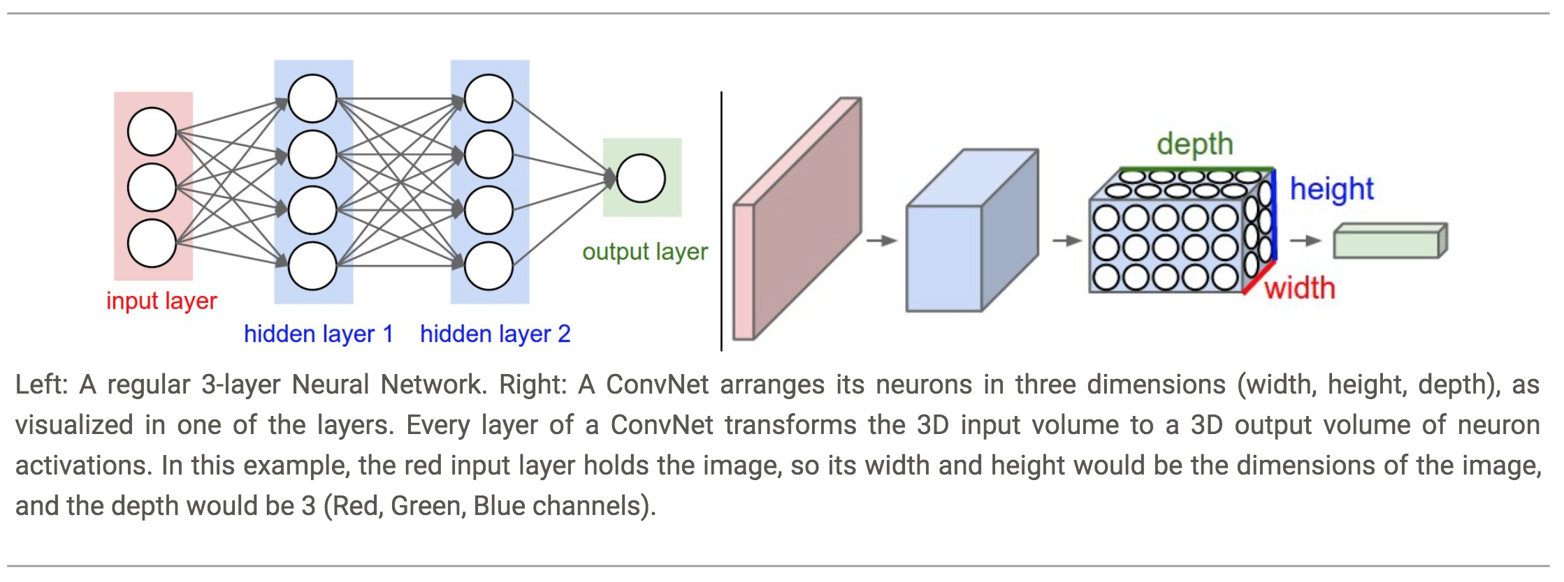
- Layers:
We use three main types of layers to build ConvNet architectures:- Convolutional Layer:
- Convolution (Linear Transformation)
- Activation (Non-Linear Transformation; e.g. ReLU)
Known as Detector Stage
- Pooling Layer
- Fully-Connected Layer
- Convolutional Layer:
-
- Process:
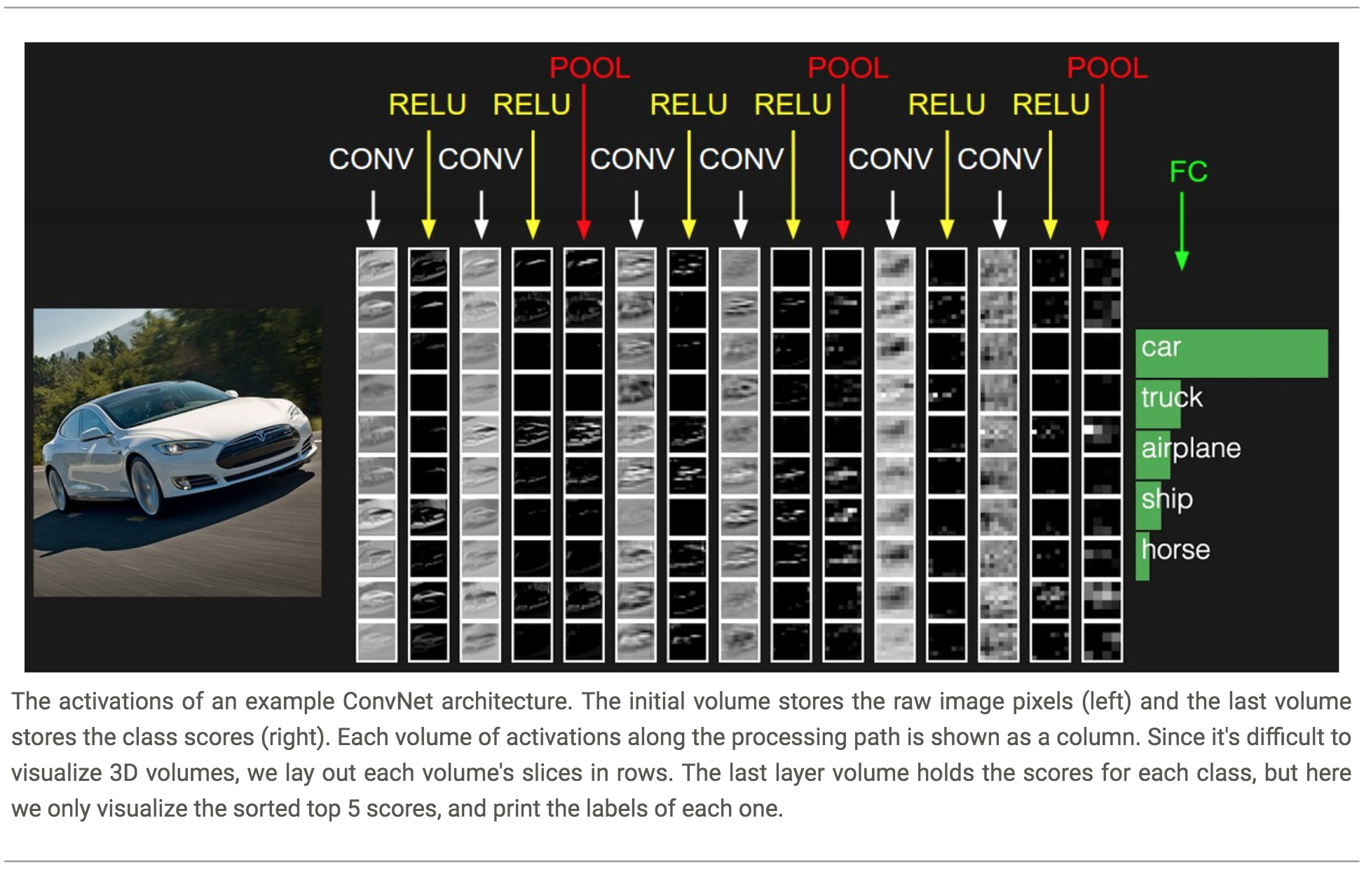
- ConvNets transform the original image layer by layer from the original pixel values to the final class scores.
-
- Example Architecture (CIFAR-10):
- Model: [INPUT - CONV - RELU - POOL - FC]
-
- INPUT: [32x32x3] will hold the raw pixel values of the image, in this case an image of width 32, height 32, and with three color channels R,G,B.
- CONV-Layer will compute the output of neurons that are connected to local regions in the input, each computing a dot product between their weights and a small region they are connected to in the input volume.
This may result in volume such as [\(32\times32\times12\)] if we decided to use 12 filters. - RELU-Layer: will apply an element-wise activation function, thresholding at zero. This leaves the size of the volume unchanged ([\(32\times32\times12\)]).
- POOL-Layer: will perform a down-sampling operation along the spatial dimensions (width, height), resulting in volume such as [\(16\times16\times12\)].
- Fully-Connected: will compute the class scores, resulting in volume of size [\(1\times1\times10\)], where each of the 10 numbers correspond to a class score, such as among the 10 categories of CIFAR-10.
As with ordinary Neural Networks and as the name implies, each neuron in this layer will be connected to all the numbers in the previous volume.
-
- Fixed Functions VS Hyper-Parameters:
- Some layers contain parameters and other don’t.
-
- CONV/FC layers perform transformations that are a function of not only the activations in the input volume, but also of the parameters (the weights and biases of the neurons).
-
- RELU/POOL layers will implement a fixed function.
-
The parameters in the CONV/FC layers will be trained with gradient descent so that the class scores that the ConvNet computes are consistent with the labels in the training set for each image.
- Summary:
- A ConvNet architecture is in the simplest case a list of Layers that transform the image volume into an output volume (e.g. holding the class scores)
- There are a few distinct types of Layers (e.g. CONV/FC/RELU/POOL are by far the most popular)
- Each Layer accepts an input 3D volume and transforms it to an output 3D volume through a differentiable function
- Each Layer may or may not have parameters (e.g. CONV/FC do, RELU/POOL don’t)
- Each Layer may or may not have additional hyperparameters (e.g. CONV/FC/POOL do, RELU doesn’t)
The Convolutional Layer

N.B.: Blue maps are inputs, and cyan maps are outputs.
| No padding, no strides | Arbitrary padding, no strides | Half padding, no strides | Full padding, no strides |
 |
 |
 |
 |
| No padding, strides | Padding, strides | Padding, strides (odd) | |
 |
 |
 |
| No padding, no strides, transposed | Arbitrary padding, no strides, transposed | Half padding, no strides, transposed | Full padding, no strides, transposed |
 |
 |
 |
 |
| No padding, strides, transposed | Padding, strides, transposed | Padding, strides, transposed (odd) | |
 |
 |
 |
| No padding, no stride, dilation |
 |
-
Convolutions:
In its most general form, the convolution is a Linear Operation on two functions of real-valued arguments.Mathematically, a Convolution is a mathematical operation on two functions (\(f\) and \(g\)) to produce a third function, that is typically viewed as a modified version of one of the original functions, giving the integral of the point-wise multiplication of the two functions as a function of the amount that one of the original functions is translated.
The convolution could be thought of as a weighting function (e.g. for taking the weighted average of a series of numbers/function-outputs).The convolution of the continuous functions \(f\) and \(g\):
$${\displaystyle {\begin{aligned}(f * g)(t)&\,{\stackrel {\mathrm {def} }{=}}\ \int _{-\infty }^{\infty }f(\tau )g(t-\tau )\,d\tau \\&=\int_{-\infty }^{\infty }f(t-\tau )g(\tau )\,d\tau .\end{aligned}}}$$
The convolution of the discreet functions f and g:
$${\displaystyle {\begin{aligned}(f * g)[n]&=\sum_{m=-\infty }^{\infty }f[m]g[n-m]\\&=\sum_{m=-\infty }^{\infty }f[n-m]g[m].\end{aligned}}} (commutativity)$$
In this notation, we refer to:
- The function \(f\) as the Input
- The function \(g\) as the Kernel/Filter
- The output of the convolution as the Feature Map
Commutativity:
Can be achieved by flipping the kernel with respect to the input; in the sense that as increases, the index into the \(m\) input increases, but the index into the kernel decreases.
While the commutative property is useful for writing proofs, it is not usually an important property of a neural network implementation.
Moreover, in a CNN, the convolution is used simultaneously with other functions, and the combination of these functions does not commute regardless of whether the convolution operation flips its kernel or not.
Because Convolutional networks usually use multichannel convolution, the linear operations they are based on are not guaranteed to be commutative, even if kernel flipping is used. These multichannel operations are only commutative if each operation has the same number of output channels as input channels.Motivation:
The convolution operation can be used to compute many results in different domains. It originally arose in pure mathematics and probability theory as a way to combine probability distributions.Understanding the Convolution Operation:
-
It can be seen as a sliding window of multiplying the values from one array with the other array. It can also be seen as a matrix generated by the outer product of the two “vectors” and then summing the diagonals.
-
The \(n\)th element of the convolution is the sum of the product of the elements in the two arrays such that the indices of the arrays sum up to \(n\):

The formula for the convolution of \(a\) and \(b\):
$$(a * b)_n=\sum_{\substack{i, j \\ i+j=n}} a_i \cdot b_j$$
Where does it apply?
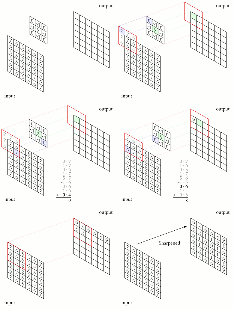
- Image Processing: different kernels give us different image processing effects like the examples below.
- Image Blurring: calculating a 2d moving average of the image results in a form of blurring.


- Vertical Edge Detection:


- Horizontal Edge Detection:


- Image Sharpening:


- Image Blurring: calculating a 2d moving average of the image results in a form of blurring.
- Probability:
- Sum of two Probability Distributions: the convolution of the probabilities of each event corresponds to adding two probability distributions together \(P_{X+Y}\):

- Calculating a moving average (equivalently, data smoothing):


- Sum of two Probability Distributions: the convolution of the probabilities of each event corresponds to adding two probability distributions together \(P_{X+Y}\):
- Differential Equations: solving DEs
- Polynomials: in multiplying two polynomials, the coeffecients are the convolution of the coeffecients of the original polynomials (which are the sums of the diagonals of the convolution matrix):

- Multiplication of two numbers:

Computing the Convolution Operation:
We can compute the convolution of two arrays much faster by utilizing the FFT algorithm as implemented by thescipy.signal.fftconvolvefunction.
Deriving the faster algorithm for computing the convolution operation:
- We utilize the connection between multiplication and convolutions to come up with a faster algorithm for computing the convolution
- New Algorithm for computing the convolution of two arrays \(a, b\) (\(\mathcal{O}(N^2)\)):
- Assume the Arrays are coeffecients of two polynomials:
- Sample the polynomials at len(\(a\)), len(\(b\)) points respectively:
- Multiply the samples pointwise
- Solve the new system to recover the coeffecients which will be the convolution of \(a, b\)
Problems with this approach:
- Multiplying two polynomials by expanding the products is an \(\mathcal{O}(n^2)\) algorithm.

Key Ideas for the solution:
- Recovering a polynomial of order \(n\) only requires \(n+1\) samples
- Utilize the connection between multiplication of polynomials and convolutions I.E. we can translate one problem into the other.
-
Utilize the Discrete Fourier Transform (DFT) of the coeffecients to compute the samples of each constructed polynomial to reduce the runtime from \(\mathcal{O}(N^2)\) to \(\mathcal{O}(N \log(N))\)

Fast Convolution Algorithm using the Fast Fourier Transform (FFT) \(\mathcal{O}(N \log(N))\):
- Compute the FFT of each array (as coeffecients)
I.E. Treat them as polynomials and evaluate them at the roots of unity

- Multiply the FFT of each array, pointwise

- Compute the inverse FFT of the new result of multiplication

Key Results:
The connection between all these applications of Convolutions, and its’ connection to the FFT implies that we can compute all the results above in \(\mathcal{O}(N \log(N))\) time (e.g. sum of probabilities, image processing, etc.). -
- Cross-Correlation:
- Cross-Correlation is a measure of similarity of two series as a function of the displacement of one relative to the other.
- The continuous cross-correlation on continuous functions f and g:
- \[(f\star g)(\tau )\ {\stackrel {\mathrm {def} }{=}}\int_{-\infty }^{\infty }f^{*}(t)\ g(t+\tau )\,dt,\]
- The discrete cross-correlation on discreet functions f and g:
-
$$(f\star g)[n]\ {\stackrel {\mathrm {def} }{=}}\sum _{m=-\infty }^{\infty }f^{*}[m]\ g[m+n].$$
- Convolutions and Cross-Correlation:
- Convolution is similar to cross-correlation.
- For discrete real valued signals, they differ only in a time reversal in one of the signals.
- For continuous signals, the cross-correlation operator is the adjoint operator of the convolution operator.
-
CNNs, Convolutions, and Cross-Correlation:
The term Convolution in the name “Convolution Neural Network” is unfortunately a misnomer.
CNNs actually use Cross-Correlation instead as their similarity operator.
The term ‘convolution’ has stuck in the name by convention.
- Convolution in DL:
The Convolution operation:$$s(t)=(x * w)(t)=\sum_{a=-\infty}^{\infty} x(a) w(t-a)$$
we usually assume that these functions are zero everywhere but in the finite set of points for which we store the values.
- Convolution Over Two Axis:
If we use a 2D image \(I\) as our input, we probably also want to use a two-dimensional kernel \(K\):$$S(i, j)=(I * K)(i, j)=\sum_{m} \sum_{n} I(m, n) K(i-m, j-n)$$
In practice we use the following formula instead (commutativity):
$$S(i, j)=(K * I)(i, j)=\sum_{m} \sum_{n} I(i-m, j-n) K(m, n)$$
Usually the latter formula is more straightforward to implement in a machine learning library, because there is less variation in the range of valid values of \(m\) and \(n\).
The Cross-Correlation is usually implemented by ML-libs:
$$S(i, j)=(K * I)(i, j)=\sum_{m} \sum_{n} I(i+m, j+n) K(m, n)$$

- The Mathematics of the Convolution Operation:
- The operation can be broken into matrix multiplications using the Toeplitz matrix representation for 1D and block-circulant matrix for 2D convolution:
- Discrete convolution can be viewed as multiplication by a matrix, but the matrix has several entries constrained to be equal to other entries.
For example, for univariate discrete convolution, each row of the matrix is constrained to be equal to the row above shifted by one element. This is known as a Toeplitz matrix.
A Toeplitz matrix has the property that values along all diagonals are constant.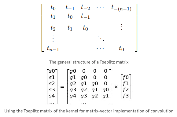
- In two dimensions, a doubly block circulant matrix corresponds to convolution.
A matrix which is circulant with respect to its sub-matrices is called a block circulant matrix. If each of the submatrices is itself circulant, the matrix is called doubly block-circulant matrix.

- Discrete convolution can be viewed as multiplication by a matrix, but the matrix has several entries constrained to be equal to other entries.
- Convolution usually corresponds to a very sparse matrix (a matrix whose entries are mostly equal to zero).
This is because the kernel is usually much smaller than the input image. - Any neural network algorithm that works with matrix multiplication and does not depend on specific properties of the matrix structure should work with convolution, without requiring any further changes to the neural network.
- Typical convolutional neural networks do make use of further specializations in order to deal with large inputs efficiently, but these are not strictly necessary from a theoretical perspective.
- The operation can be broken into matrix multiplications using the Toeplitz matrix representation for 1D and block-circulant matrix for 2D convolution:
- The Convolution operation in a CONV Layer:
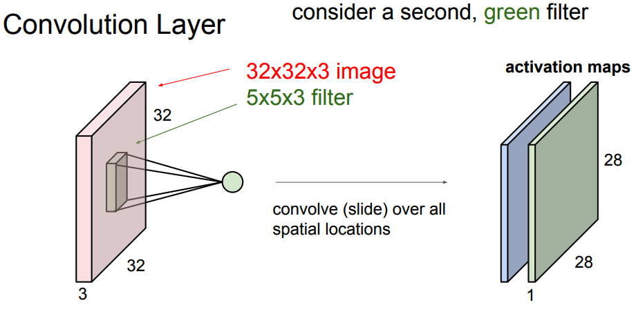
- The CONV layer’s parameters consist of a set of learnable filters.
- Every filter is small spatially (along width and height), but extends through the full depth of the input volume.
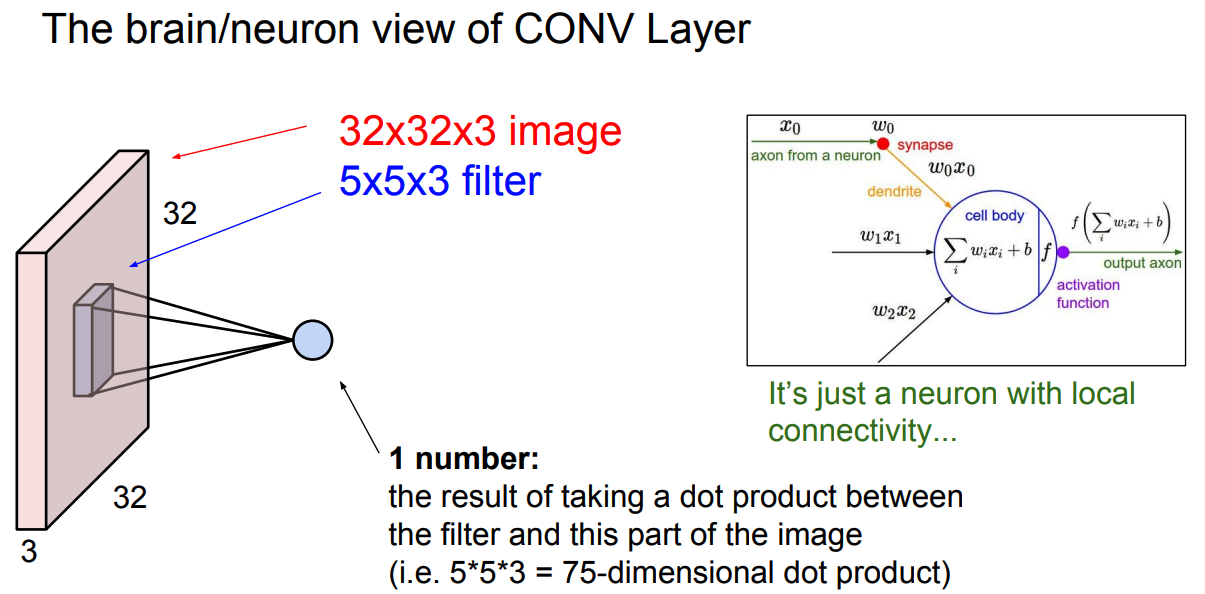
For example, a typical filter on a first layer of a ConvNet might have size 5x5x3 (i.e. 5 pixels width and height, and 3 because images have depth 3, the color channels).
- Every filter is small spatially (along width and height), but extends through the full depth of the input volume.
- In the forward pass, we slide (convolve) each filter across the width and height of the input volume and compute dot products between the entries of the filter and the input at any position.
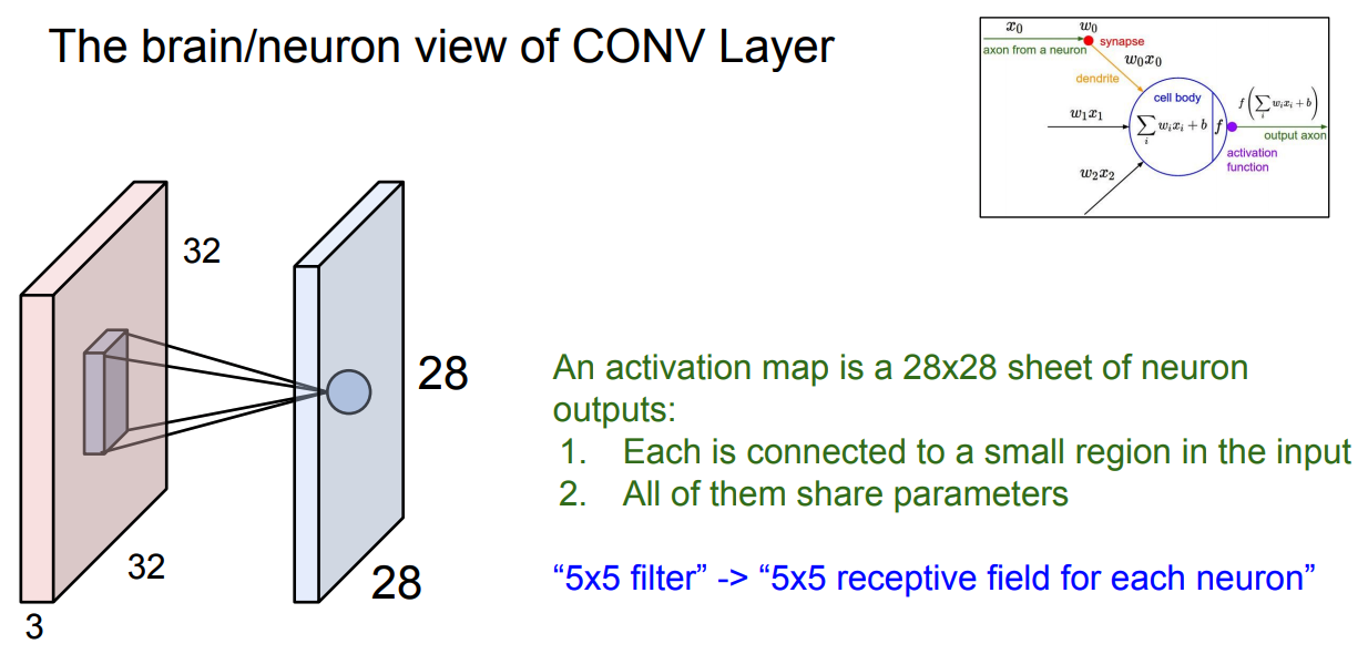
- As we slide the filter over the width and height of the input volume we will produce a 2-dimensional activation map that gives the responses of that filter at every spatial position.
Intuitively, the network will learn filters that activate when they see some type of visual feature such as an edge of some orientation or a blotch of some color on the first layer, or eventually entire honeycomb or wheel-like patterns on higher layers of the network.
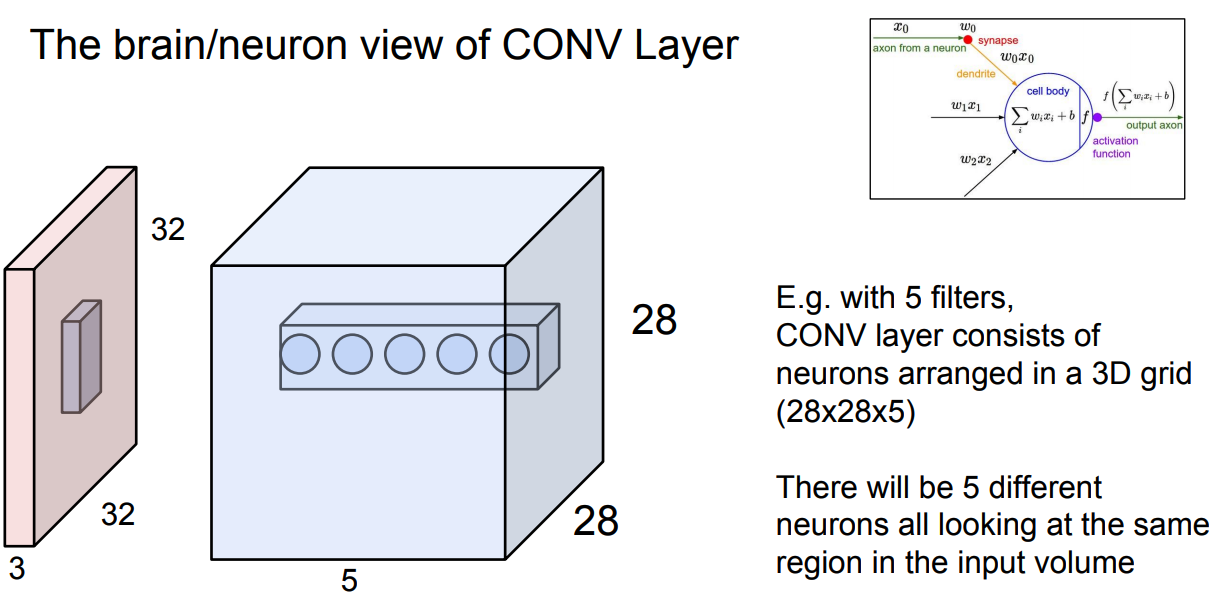
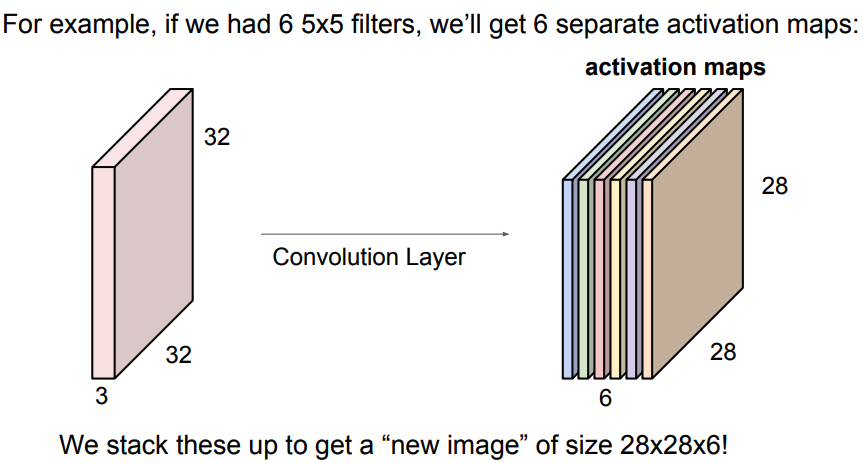
- Now, we will have an entire set of filters in each CONV layer (e.g. 12 filters), and each of them will produce a separate 2-dimensional activation map.
- We will stack these activation maps along the depth dimension and produce the output volume.
- As we slide the filter over the width and height of the input volume we will produce a 2-dimensional activation map that gives the responses of that filter at every spatial position.
As a result (of what?), the network learns filters that activate when it detects some specific type of feature at some spatial position in the input.
- The CONV layer’s parameters consist of a set of learnable filters.
-
The Brain Perspective:
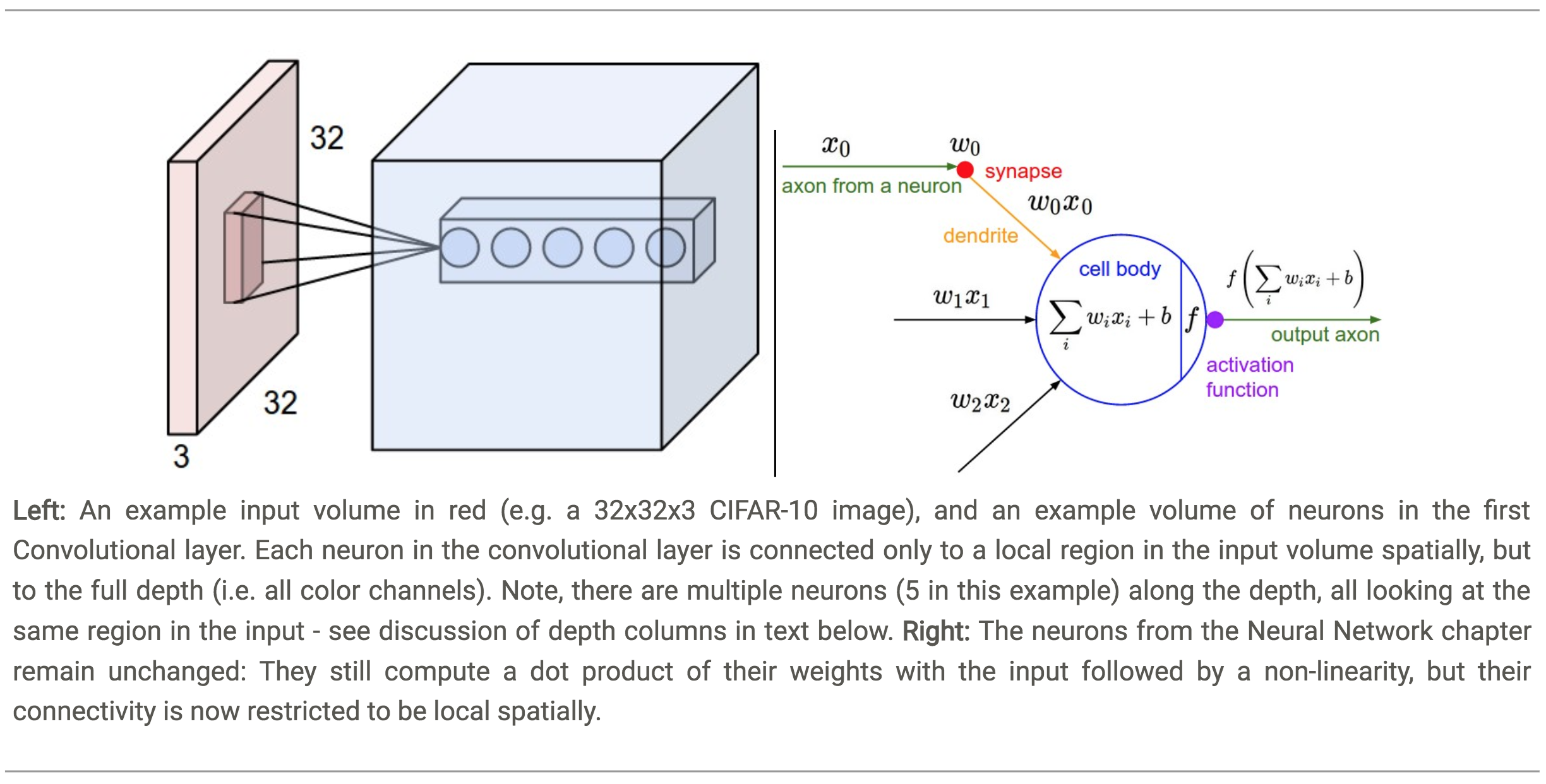
Every entry in the 3D output volume can also be interpreted as an output of a neuron that looks at only a small region in the input and shares parameters with all neurons to the left and right spatially.
- Local Connectivity:
- Convolutional networks exploit spatially local correlation by enforcing a local connectivity pattern between neurons of adjacent layers:
- Each neuron is connected to only a small region of the input volume.
- The Receptive Field of the neuron defines the extent of this connectivity as a hyperparameter.
For example, suppose the input volume has size \([32\times32\times3]\) and the receptive field (or the filter size) is \(5\times5\), then each neuron in the Conv Layer will have weights to a \([5\times5\times3]\) region in the input volume, for a total of \(5*5*3 = 75\) weights (and \(+1\) bias parameter).
Such an architecture ensures that the learnt filters produce the strongest response to a spatially local input pattern.
- Convolutional networks exploit spatially local correlation by enforcing a local connectivity pattern between neurons of adjacent layers:
- Spatial Arrangement:
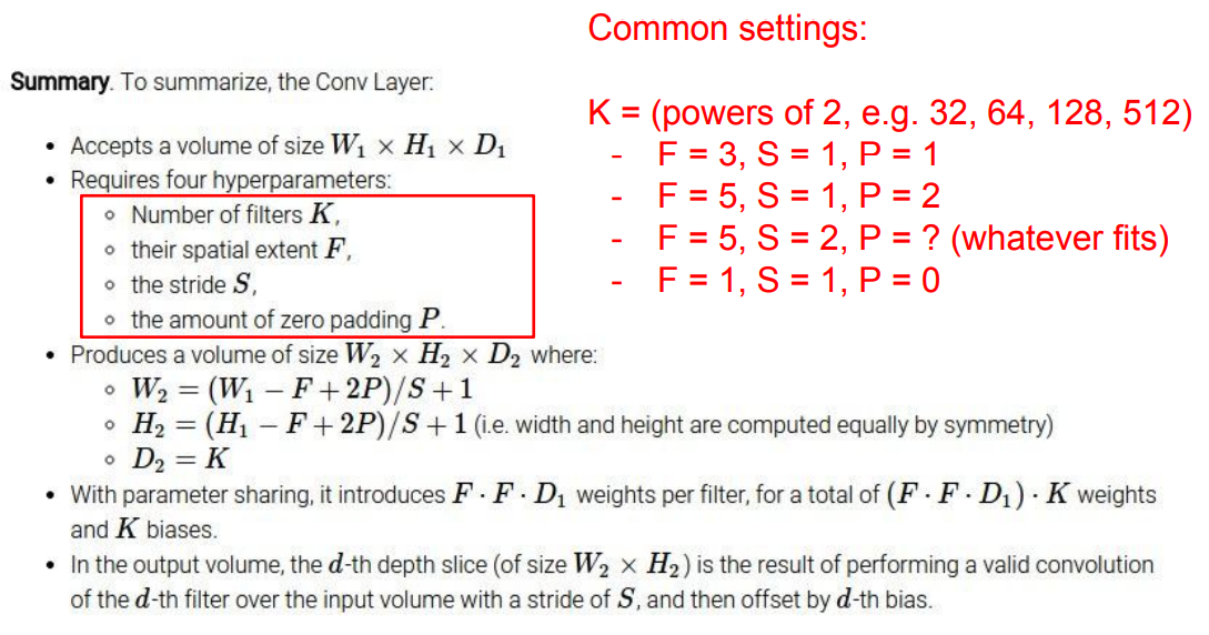
There are three hyperparameters control the size of the output volume:- The Depth of the output volume is a hyperparameter that corresponds to the number of filters we would like to use (each learning to look for something different in the input).
- The Stride controls how depth columns around the spatial dimensions (width and height) are allocated.
e.g. When the stride is 1 then we move the filters one pixel at a time.
- The Smaller the stride, the more overlapping regions exist and the bigger the volume.
- The bigger the stride, the less overlapping regions exist and the smaller the volume.
- The Padding is a hyperparameter whereby we pad the input volume with zeros around the border.
This allows to control the spatial size of the output volumes.
- The Spatial Size of the Output Volume:
We compute the spatial size of the output volume as a function of:- \(W\): The input volume size.
- \(F\): \(\:\)The receptive field size of the Conv Layer neurons.
- \(S\): \(\:\)The stride with which they are applied.
- \(P\): \(\:\)The amount of zero padding used on the border.
Thus, the Total Size of the Output:
$$\dfrac{W−F+2P}{S} + 1$$
Potential Issue: If this number is not an integer, then the strides are set incorrectly and the neurons cannot be tiled to fit across the input volume in a symmetric way.
- Fix: In general, setting zero padding to be \({\displaystyle P = \dfrac{K-1}{2}}\) when the stride is \({\displaystyle S = 1}\) ensures that the input volume and output volume will have the same size spatially.
- Calculating the Number of Parameters:
Given:- Input Volume: \(32\times32\times3\)
- Filters: \(10\:\:\: (5\times5)\)
- Stride: \(1\)
- Pad: \(2\)
The number of parameters equals the number of parameters in each filter \(= 5*5*3 + 1 = 76\) (+1 for bias) times the number of filters \(76 * 10 = 760\).
-
The Convolution Layer:
__
__The Conv Layer and the Brain:
__
__
__
-
From FC-layers to Conv-layers:
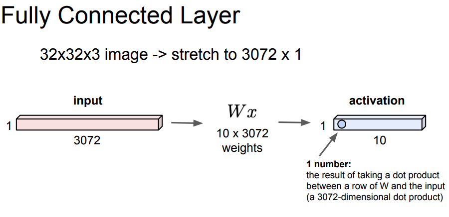
**
**
*** -
\(1\times1\) Convolutions:
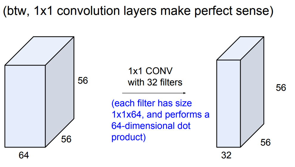
- Notes:
- Summary:
- ConvNets stack CONV,POOL,FC layers
- Trend towards smaller filters and deeper architectures
- Trend towards getting rid of POOL/FC layers (just CONV)
- Typical architectures look like [(CONV-RELU) * N-POOL?] * M-(FC-RELU) * K, SOFTMAX
where \(N\) is usually up to ~5, \(M\) is large, \(0 <= K <= 2\).
But recent advances such as ResNet/GoogLeNet challenge this paradigm
- Effect of Different Biases:
Separating the biases may slightly reduce the statistical efficiency of the model, but it allows the model to correct for differences in the image statistics at different locations. For example, when using implicit zero padding, detector units at the edge of the image receive less total input and may need larger biases. - In the kinds of architectures typically used for classification of a single object in an image, the greatest reduction in the spatial dimensions of the network comes from using pooling layers with large stride.
- Summary:
The Pooling Layer
-
The Pooling Operation/Function:
The pooling function calculates a summary statistic of the nearby pixels at the point of operation.
Some common statistics are max, mean, weighted average and \(L^2\) norm of a surrounding rectangular window.
- The Key Ideas/Properties:
In all cases, pooling helps to make the representation approximately invariant to small translations of the input.Invariance to translation means that if we translate the input by a small amount, the values of most of the pooled outputs do not change.
Invariance to local translation can be a useful property if we care more about whether some feature is present than exactly where it is.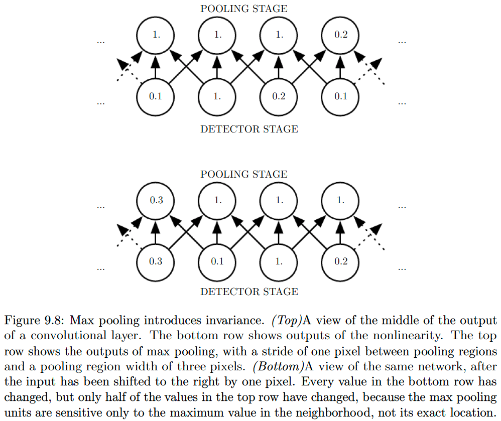
(Learned) Invariance to other transformations:
Pooling over spatial regions produces invariance to translation, but if we pool over the outputs of separately parametrized convolutions, the features can learn which transformations to become invariant to.
This property has been used in Maxout networks.
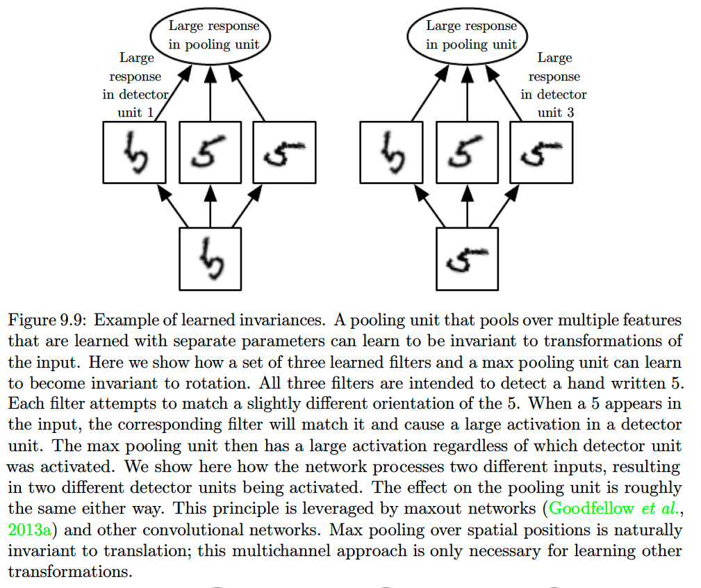
For many tasks, pooling is essential for handling inputs of varying size.
This is usually accomplished by varying the size of an offset between pooling regions so that the classification layer always receives the same number of summary statistics regardless of the input size. For example, the final pooling layer of the network may be defined to output four sets of summary statistics, one for each quadrant of an image, regardless of the image size.
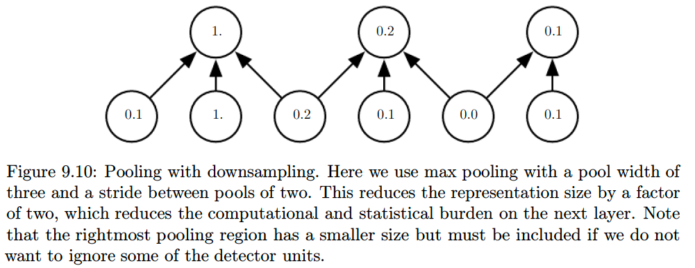
One can use fewer pooling units than detector units, since they provide a summary; thus, by reporting summary statistics for pooling regions spaced \(k\) pixels apart rather than \(1\) pixel apart, we can improve the computational efficiency of the network because the next layer has roughly \(k\) times fewer inputs to process.
This reduction in the input size can also result in improved statistical efficiency and reduced memory requirements for storing the parameters.
-
Theoretical Guidelines for choosing the pooling function:
Link
-
Variations:
Dynamical Pooling:
It is also possible to dynamically pool features together, for example, by running a clustering algorithm on the locations of interesting features (Boureau et al., 2011) link. This approach yields a different set of pooling regions for each image.Learned Pooling:
Another approach is to learn a single pooling structure that is then applied to all images (Jia et al., 2012).
-
Pooling and Top-Down Architectures:
Pooling can complicate some kinds of neural network architectures that use top-down information, such as Boltzmann machines and autoencoders.
- The Pooling Layer (summary):
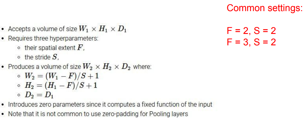
Notes:
- Pooling Layer:
- Makes the representations smaller and more manageable
- Operates over each activation map independently (i.e. preserves depth)
- You can use the stride instead of the pooling to downsample
Convolution and Pooling as an Infinitely Strong Prior
-
A Prior Probability Distribution:
This is a probability distribution over the parameters of a model that encodes our beliefs about what models are reasonable, before we have seen any data.
- What is a weight prior?:
Assumptions about the weights (before learning) in terms of acceptable values and range are encoded into the prior distribution of the weights.- A Weak Prior: has a high entropy, and thus, variance and shows that there is low confidence in the initial value of the weight.
- A Strong Prior: in turn has low entropy/variance, and shows a narrow range of values about which we are confident before learning begins.
- A Infinitely Strong Prior: demarkets certain values as forbidden completely, assigning them zero probability.
- Convolutional Layer as a FC Layer:
If we view the conv-layer as a FC-layer, the:- Convolution: operation imposes an infinitely strong prior by making the following restrictions on the weights:
- Adjacent units must have the same weight but shifted in space.
- Except for a small spatially connected region, all other weights must be zero.
- Pooling: operation imposes an infinitely strong prior by:
- Requiring features to be Translation Invariant.
- Requiring features to be Translation Invariant.
- Convolution: operation imposes an infinitely strong prior by making the following restrictions on the weights:
- Key Insights/Takeaways:
- Convolution and pooling can cause underfitting if the priors imposed are not suitable for the task. When a task involves incorporating information from very distant locations in the input, then the prior imposed by convolution may be inappropriate.
As an example, consider this scenario. We may want to learn different features for different parts of an input. But the compulsion to used tied weights (enforced by standard convolution) on all parts of an image, forces us to either compromise or use more kernels (extract more features).
- Convolutional models should only be compared with other convolutional models. This is because other models which are permutation invariant can learn even when input features are permuted (thus loosing spatial relationships). Such models need to learn these spatial relationships (which are hard-coded in CNNs).
- Convolution and pooling can cause underfitting if the priors imposed are not suitable for the task. When a task involves incorporating information from very distant locations in the input, then the prior imposed by convolution may be inappropriate.
Variants of the Basic Convolution Function and Structured Outputs
- Practical Considerations for Implementing the Convolution Function:
- In general a convolution layer consists of application of several different kernels to the input. This allows the extraction of several different features at all locations in the input. This means that in each layer, a single kernel (filter) isn’t applied. Multiple kernels (filters), usually a power of 2, are used as different feature detectors.
- The input is generally not real-valued but instead vector valued (e.g. RGB values at each pixel or the feature values computed by the previous layer at each pixel position). Multi-channel convolutions are commutative only if number of output and input channels is the same.
- Strided Convolutions are a means to do DownSampling; they are used to reduce computational cost, by calculating features at a coarser level. The effect of strided convolution is the same as that of a convolution followed by a downsampling stage. This can be used to reduce the representation size.
$$Z_{i, j, k}=c(\mathrm{K}, \mathrm{V}, s)_{i, j, k}=\sum_{l, m, n}\left[V_{l,(j-1) \times s+m,(k-1) \times s+n} K_{i, l, m, n}\right] \tag{9.8}$$
- Zero Padding is used to make output dimensions and kernel size independent (i.e. to control the output dimension regardless of the size of the kernel). There are three types:
- Valid: The output is computed only at places where the entire kernel lies inside the input. Essentially, no zero padding is performed. For a kernel of size \(k\) in any dimension, the input shape of \(m\) in the direction will become \(m-k+1\) in the output. This shrinkage restricts architecture depth.
- Same: The input is zero padded such that the spatial size of the input and output is same. Essentially, for a dimension where kernel size is \(k\), the input is padded by \(k-1\) zeros in that dimension. Since the number of output units connected to border pixels is less than that for center pixels, it may under-represent border pixels.
- Full: The input is padded by enough zeros such that each input pixel is connected to the same number of output units.
The optimal amount of Zero-Padding usually lies between “valid” and “same” convolution.
- Locally Connected Layers/Unshared Convolution: has the same connectivity graph as a convolution operation, but without parameter sharing (i.e. each output unit performs a linear operation on its neighbourhood but the parameters are not shared across output units.).
This allows models to capture local connectivity while allowing different features to be computed at different spatial locations; at the expense of having a lot more parameters.$$Z_{i, j, k}=\sum_{l, m, n}\left[V_{l, j+m-1, k+n-1} w_{i, j, k, l, m, n}\right] \tag{9.9}$$
They’re useful when we know that each feature should be a function of a small part of space, but there is no reason to think that the same feature should occur across all of space.
For example, if we want to tell if an image is a picture of a face, we only need to look for the mouth in the bottom half of the image. - Tiled Convolution: offers a middle ground between Convolution and locally-connected layers. Rather than learning a separate set of weights at every spatial location, it learns/uses a set of kernels that are cycled through as we move through space.
This means that immediately neighboring locations will have different filters, as in a locally connected layer, but the memory requirements for storing the parameters will increase only by a factor of the size of this set of kernels, rather than by the size of the entire output feature map.$$Z_{i, j, k}=\sum_{l, m, n} V_{l, j+m-1, k+n-1} K_{i, l, m, n, j \% t+1, k \% t+1} \tag{9.10}$$
- Max-Pooling, and Locally Connected Layers and Tiled Layers: When max pooling operation is applied to locally connected layer or tiled convolution, the model has the ability to become transformation invariant because adjacent filters have the freedom to learn a transformed version of the same feature.
This essentially similar to the property leveraged by pooling over channels rather than spatially.
- Different Connections: Besides locally-connected layers and tiled convolution, another extension can be to restrict the kernels to operate on certain input channels. One way to implement this is to connect the first m input channels to the first n output channels, the next m input channels to the next n output channels and so on. This method decreases the number of parameters in the model without decreasing the number of output units.
- Other Operations: The following three operations—convolution, backprop from output to weights, and backprop from output to inputs—are sufficient to compute all the gradients needed to train any depth of feedforward convolutional network, as well as to train convolutional networks with reconstruction functions based on the transpose of convolution.
See Goodfellow (2010) for a full derivation of the equations in the fully general multidimensional, multiexample case.
- Bias: Bias terms can be used in different ways in the convolution stage.
- For locally connected layer and tiled convolution, we can use a bias per output unit and kernel respectively.
- In case of traditional convolution, a single bias term per output channel is used.
- If the input size is fixed, a bias per output unit may be used to counter the effect of regional image statistics and smaller activations at the boundary due to zero padding.
- Structured Outputs:
Convolutional networks can be trained to output high-dimensional structured output rather than just a classification score.
A good example is the task of image segmentation where each pixel needs to be associated with an object class.
Here the output is the same size (spatially) as the input. The model outputs a tensor \(S\) where \(S_{i, j, k}\) is the probability that pixel \((j,k)\) belongs to class \(i\).- Problem: One issue that often comes up is that the output plane can be smaller than the input plane.
- Solutions:
- To produce an output map as the same size as the input map, only same-padded convolutions can be stacked.
- Avoid Pooling Completely (Jain et al. 2007)
- Emit a lower-Resolution grid of labels (Pinheiro and Collobert, 2014, 2015)
- Recurrent-Convolutional Models: The output of the first labelling stage can be refined successively by another convolutional model. If the models use tied parameters, this gives rise to a type of recursive model.
- Another model that has gained popularity for segmentation tasks (especially in the medical imaging community) is the U-Net. The up-convolution mentioned is just a direct upsampling by repetition followed by a convolution with same padding.
The output can be further processed under the assumption that contiguous regions of pixels will tend to belong to the same label. Graphical models can describe this relationship. Alternately, CNNs can learn to optimize the graphical models training objective.
Extra
-
- Image Features:
- are certain quantities that are calculated from the image to better describe the information in the image, and to reduce the size of the input vectors.
-
- Examples:
- Color Histogram: Compute a (bucket-based) vector of colors with their respective amounts in the image.
- Histogram of Oriented Gradients (HOG): we count the occurrences of gradient orientation in localized portions of the image.
- Bag of Words: a bag of visual words is a vector of occurrence counts of a vocabulary of local image features.
The visual words can be extracted using a clustering algorithm; K-Means.
- Examples: