Ahmad Badary

Introduction

Introduction

Recurrent Neural Networks:
Recurrent Neural Networks (RNNs) are a family of neural networks for processing sequential data.

In an RNN, the connections between units form a directed cycle, allowing it to exhibit dynamic temporal behavior.

The standard RNN is a nonlinear dynamical system that maps sequences to sequences.
Big Idea:
RNNs share parameters across different positions/index of time/time-steps of the sequence, which allows it to generalize well to examples of different sequence length.
- Such sharing is particularly important when a specific piece of information can occur at multiple positions within the sequence.
A related idea, is the use of convolution across a 1-D temporal sequence (time-delay NNs). This convolution operation allows the network to share parameters across time but is shallow.
The output of convolution is a sequence where each member of the output is a function of a small number of neighboring members of the input.
Dynamical Systems:
A Dynamical System is a system in which a function describes the time dependence of a point in a geometrical space.

Classical Form of a Dynamical System:

$$\boldsymbol{s}^{(t)}=f\left(\boldsymbol{s}^{(t-1)} ; \boldsymbol{\theta}\right) \tag{10.1}$$

where $\boldsymbol{s}^{(t)}$ is called the state of the system.

A Dynamical System driven by an external signal $\boldsymbol{x}^{(t)}$:

$$\boldsymbol{s}^{(t)}=f\left(\boldsymbol{s}^{(t-1)}, \boldsymbol{x}^{(t)} ; \boldsymbol{\theta}\right) \tag{10.4}$$

the state now contains information about the whole past sequence.

Basically, any function containing recurrence can be considered an RNN.

The RNN Equation (as a Dynamical System):

$$\boldsymbol{h}^{(t)}=f\left(\boldsymbol{h}^{(t-1)}, \boldsymbol{x}^{(t)} ; \boldsymbol{\theta}\right) \tag{10.5}$$

where the variable $\mathbf{h}$ represents the state.
- Dynamical Systems (wiki!)
Unfolding the Computation Graph:
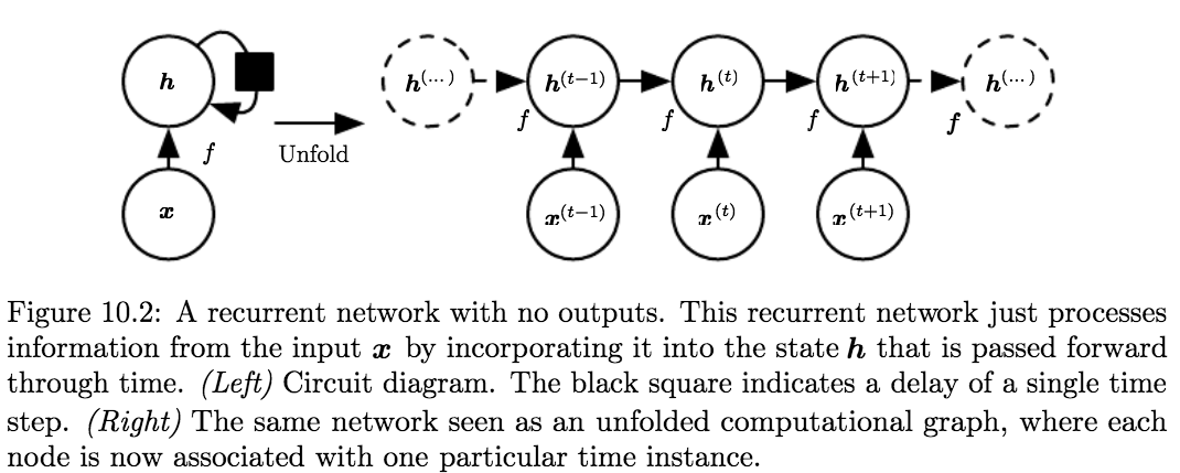
Unfolding maps the left to the right in the figure below (from figure 10.2) (both are computational graphs of a RNN without output $\mathbf{o}$):

where the black square indicates that an interaction takes place with a delay of $1$ time step, from the state at time $t$ to the state at time $t + 1$.

We can represent the unfolded recurrence after $t$ steps with a function $g^{(t)}$:

$$\begin{aligned} \boldsymbol{h}^{(t)} &=g^{(t)}\left(\boldsymbol{x}^{(t)}, \boldsymbol{x}^{(t-1)}, \boldsymbol{x}^{(t-2)}, \ldots, \boldsymbol{x}^{(2)}, \boldsymbol{x}^{(1)}\right) \\ &=f\left(\boldsymbol{h}^{(t-1)}, \boldsymbol{x}^{(t)} ; \boldsymbol{\theta}\right) \end{aligned}$$

The function $g^{(t)}$ takes the whole past sequence $\left(\boldsymbol{x}^{(t)}, \boldsymbol{x}^{(t-1)}, \boldsymbol{x}^{(t-2)}, \ldots, \boldsymbol{x}^{(2)}, \boldsymbol{x}^{(1)}\right)$ as input and produces the current state, but the unfolded recurrent structure allows us to factorize $g^{(t)}$ into repeated applications of a function $f$.

The unfolding process, thus, introduces two major advantages:
1. Regardless of the sequence length, the learned model always has the same input size.
  Because it is specified in terms of transition from one state to another state, rather than specified in terms of a variable-length history of states.
2. It is possible to use the same transition function $f$ with the same parameters at every time step.
  Thus, we can learn a single shared model $f$ that operates on all time steps and all sequence lengths, rather than needing to learn a separate model $g^{(t)}$ for all possible time steps
Benefits:
- Allows generalization to sequence lengths that did not appear in the training set
- Enables the model to be estimated to be estimated with far fewer training examples than would be required without parameter sharing.
The State of the RNN $\mathbf{h}^{(t)}$:
The network typically learns to use $\mathbf{h}^{(t)}$ as a kind of lossy summary of the task-relevant aspects of the past sequence of inputs up to $t$.
This summary is, in general, necessarily lossy, since it maps an arbitrary length sequence $\left(\boldsymbol{x}^{(t)}, \boldsymbol{x}^{(t-1)}, \boldsymbol{x}^{(t-2)}, \ldots, \boldsymbol{x}^{(2)}, \boldsymbol{x}^{(1)}\right)$ to a fixed length vector $h^{(t)}$.

The most demanding situation (the extreme) is when we ask $h^{(t)}$ to be rich enough to allow one to approximately recover/reconstruct the input sequence, as in AutoEncoders.
RNN Architectures/Design Patterns:
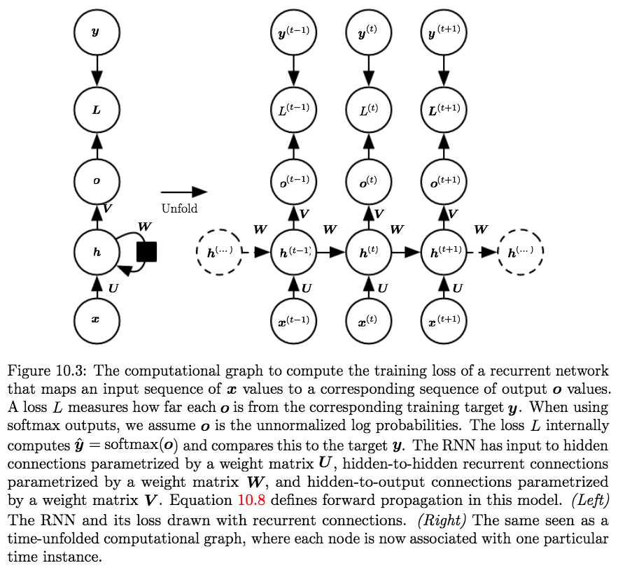
We will be introducing three variations of the RNN, and will be analyzing variation 1, the basic form of the RNN.
1. Variation 1; The Standard RNN (basic form):
  - Architecture:
    - Produces an output at each time-step
    - Recurrent connections between hidden units
  - Equations:
    The standard RNN is parametrized with three weight matrices and three bias vectors:
    $$\theta=\left[W_{h x} = U, W_{h h} = W, W_{o h} = V, b_{h}, b_{o}, h_{0}\right]$$
    
    Then given an input sequence $\left(\boldsymbol{x}^{(t)}, \boldsymbol{x}^{(t-1)}, \boldsymbol{x}^{(t-2)}, \ldots, \boldsymbol{x}^{(2)}, \boldsymbol{x}^{(1)}\right)$ the RNN performs the following computations for every time step:
    
    $$\begin{aligned} \boldsymbol{a}^{(t)} &=\boldsymbol{b}+\boldsymbol{W h}^{(t-1)}+\boldsymbol{U} \boldsymbol{x}^{(t)} \\ \boldsymbol{h}^{(t)} &=\tanh \left(\boldsymbol{a}^{(t)}\right) \\ \boldsymbol{o}^{(t)} &=\boldsymbol{c}+\boldsymbol{V} \boldsymbol{h}^{(t)} \\ \hat{\boldsymbol{y}}^{(t)} &=\operatorname{softmax}\left(\boldsymbol{o}^{(t)}\right) \end{aligned}$$
    
    where the parameters are the bias vectors $\mathbf{b}$ and $\mathbf{c}$ along with the weight matrices $\boldsymbol{U}$, $\boldsymbol{V}$ and $\boldsymbol{W}$, respectively, for input-to-hidden, hidden-to-output and hidden-to-hidden connections.
    We, also, Assume the hyperbolic tangent activation function, and that the output is discrete¹.
  - The (Total) Loss:
    The Total Loss for a given sequence of $\mathbf{x}$ values paired with a sequence of $\mathbf{y}$ values is the sum of the losses over all the time steps. Assuming $L^{(t)}$ is the negative log-likelihood of $y^{(t)}$ given $\boldsymbol{x}^{(1)}, \ldots, \boldsymbol{x}^{(t)}$, then:
    $$\begin{aligned} & L\left(\left\{\boldsymbol{x}^{(1)}, \ldots, \boldsymbol{x}^{(\tau)}\right\},\left\{\boldsymbol{y}^{(1)}, \ldots, \boldsymbol{y}^{(\tau)}\right\}\right) \\=& \sum_{t} L^{(t)} \\=& -\sum_{t} \log p_{\text { model }}\left(y^{(t)} |\left\{\boldsymbol{x}^{(1)}, \ldots, \boldsymbol{x}^{(t)}\right\}\right) \end{aligned}$$
    
    where $p_{\text { model }}\left(y^{(t)} |\left\{\boldsymbol{x}^{(1)}, \ldots, \boldsymbol{x}^{(t)}\right\}\right)$ is given by reading the entry for $y^{(t)}$ from the model’s output vector $\hat{\boldsymbol{y}}^{(t)}$.
  - Complexity:
    - Forward Pass:
      The runtime is $\mathcal{O}(\tau)$ and cannot be reduced by parallelization because the forward propagation graph is inherently sequential; each time step may only be computed after the previous one.
    - Backward Pass:
      The standard algorithm used is called Back-Propagation Through Time (BPTT), with a runtime of $\mathcal{O}(\tau)$
  - Properties:
    - The Standard RNN is Universal, in the sense that any function computable by a Turing Machine can be computed by such an RNN of a finite size.
      
      The functions computable by a Turing machine are discrete, so these results regard exact implementation of the function, not approximations.
      The RNN, when used as a Turing machine, takes a binary sequence as input, and its outputs must be discretized to provide a binary output.
    - The output can be read from the RNN after a number of time steps that is asymptotically linear in the number of time steps used by the Turing machine and asymptotically linear in the length of the input (Siegelmann and Sontag, 1991; Siegelmann, 1995; Siegelmann and Sontag, 1995; Hyotyniemi, 1996).
    - The theoretical RNN used for the proof can simulate an unbounded stack by representing its activations and weights with rational numbers of unbounded precision.
2. Variation 2:
  - Architecture:
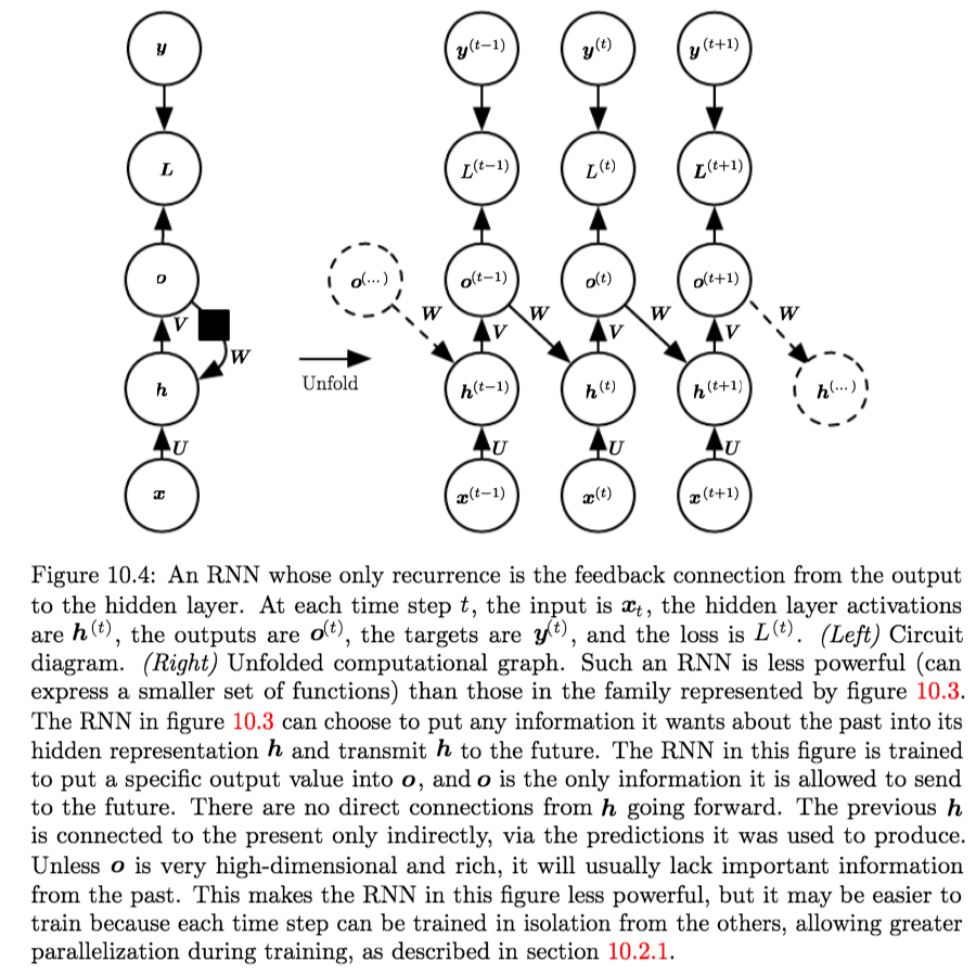
    - Produces an output at each time-step
    - Recurrent connections only from the output at one time step to the hidden units at the next time step
  - Equations:
    $$\begin{aligned} \boldsymbol{a}^{(t)} &=\boldsymbol{b}+\boldsymbol{W o}^{(t-1)}+\boldsymbol{U} \boldsymbol{x}^{(t)} \\ \boldsymbol{h}^{(t)} &=\tanh \left(\boldsymbol{a}^{(t)}\right) \\ \boldsymbol{o}^{(t)} &=\boldsymbol{c}+\boldsymbol{V} \boldsymbol{h}^{(t)} \\ \hat{\boldsymbol{y}}^{(t)} &=\operatorname{softmax}\left(\boldsymbol{o}^{(t)}\right) \end{aligned}$$
  - Properties:
    - Strictly less powerful because it lacks hidden-to-hidden recurrent connections.
      It cannot simulate a universal Turing Machine.
    - It requires that the output units capture all the information about the past that the network will use to predict the future; due to the lack of hidden-to-hidden recurrence.
      But, since the outputs are trained to match the training set targets, they are unlikely to capture the necessary information about the past history.
    - The Advantage of eliminating hidden-to-hidden recurrence is that all the time steps are de-coupled². Training can thus be parallelized, with the gradient for each step $t$ computed in isolation.
      Thus, the model can be trained with Teacher Forcing.
3. Variation 3:
  - Architecture:
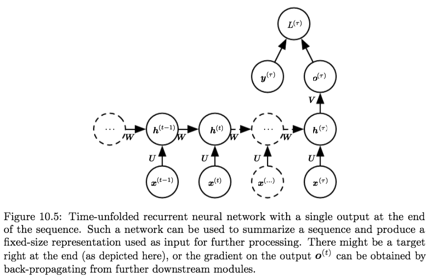
    - Produces a single output, after reading entire sequence
    - Recurrent connections between hidden units
  - Equations:
    $$\begin{aligned} \boldsymbol{a}^{(t)} &=\boldsymbol{b}+\boldsymbol{W h}^{(t-1)}+\boldsymbol{U} \boldsymbol{x}^{(t)} \\ \boldsymbol{h}^{(t)} &=\tanh \left(\boldsymbol{a}^{(t)}\right) \\ \boldsymbol{o} = \boldsymbol{o}^{(T)} &=\boldsymbol{c}+\boldsymbol{V} \boldsymbol{h}^{(T)} \\ \hat{\boldsymbol{y}} = \hat{\boldsymbol{y}}^{(T)} &=\operatorname{softmax}\left(\boldsymbol{o}^{(T)}\right) \end{aligned}$$
Teacher Forcing:
Teacher forcing is a procedure that emerges from the maximum likelihood criterion, in which during training the model receives the ground truth output $y^{(t)}$ as input at time $t + 1$.

Models that have recurrent connections from their outputs leading back into the model may be trained with teacher forcing.

Teacher forcing may still be applied to models that have hidden-to-hidden connections as long as they have connections from the output at one time step to values computed in the next time step. As soon as the hidden units become a function of earlier time steps, however, the BPTT algorithm is necessary. Some models may thus be trained with both teacher forcing and BPTT.

The disadvantage of strict teacher forcing arises if the network is going to be later used in an closed-loop mode, with the network outputs (or samples from the output distribution) fed back as input. In this case, the fed-back inputs that the network sees during training could be quite different from the kind of inputs that it will see at test time.

Methods for Mitigation:
1. Train with both teacher-forced inputs and free-running inputs, for example by predicting the correct target a number of steps in the future through the unfolded recurrent output-to-input paths³.
2. Another approach (Bengio et al., 2015b) to mitigate the gap between the inputs seen at training time and the inputs seen at test time randomly chooses to use generated values or actual data values as input. This approach exploits a curriculum learning strategy to gradually use more of the generated values as input.
proof: p.377, 378
Computing the Gradient in an RNN:

Note: The computation is, as noted before, w.r.t. the standard RNN (variation 1)

Computing the gradient through a recurrent neural network is straightforward. One simply applies the generalized back-propagation algorithm of section 6.5.6 to the unrolled computational graph. No specialized algorithms are necessary.

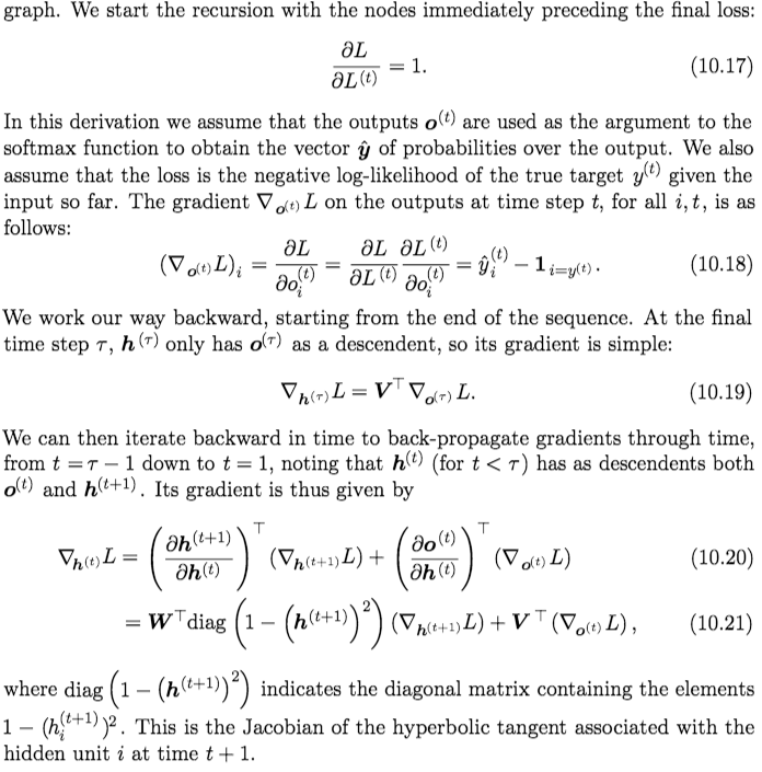
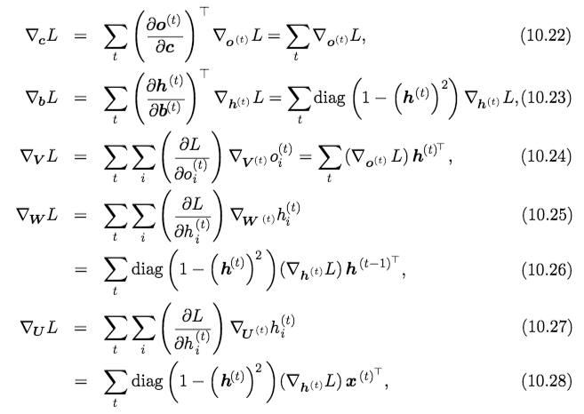
Once the gradients on the internal nodes of the computational graph are obtained, we can obtain the gradients on the parameter nodes, which have descendents at all the time steps:

Notes:
- We do not need to compute the gradient with respect to $\mathbf{x}^{(t)}$ for training because it does not have any parameters as ancestors in the computational graph defining the loss.
Recurrent Networks as Directed Graphical Models:
Since we wish to interpret the output of an RNN as a probability distribution, we usually use the cross-entropy associated with that distribution to define the loss.

E.g. Mean squared error is the cross-entropy loss associated with an output distribution that is a unit Gaussian.

When we use a predictive log-likelihood training objective, such as equation 10.12, we train the RNN to estimate the conditional distribution of the next sequence element $\boldsymbol{y}^{(t)}$ given the past inputs. This may mean that we maximize the log-likelihood:

$$\log p\left(\boldsymbol{y}^{(t)} | \boldsymbol{x}^{(1)}, \ldots, \boldsymbol{x}^{(t)}\right) \tag{10.29}$$

or, if the model includes connections from the output at one time step to the nexttime step,

$$\log p\left(\boldsymbol{y}^{(t)} | \boldsymbol{x}^{(1)}, \ldots, \boldsymbol{x}^{(t)}, \boldsymbol{y}^{(1)}, \ldots, \boldsymbol{y}^{(t-1)}\right) \tag{10.30}$$

Decomposing the joint probability over the sequence of $\mathbf{y}$ values as a series of one-step probabilistic predictions is one way to capture the full joint distribution across the whole sequence. When we do not feed past $\mathbf{y}$ values as inputs that condition the next step prediction, the outputs $\mathbf{y}$ are conditionally independent given the sequence of $\mathbf{x}$ values.

Summary:
This section is useful for understanding RNN from a probabilistic graphical model perspective. The main point is to show that RNN provides a very efficient parametrization of the joint distribution over the observations $y^{(t)}$.
The introduction of hidden state and hidden-to-hidden connections can be motivated as reducing fig 10.7 to fig 10.8; which have $\mathcal{O}(k^{\tau})$ and $\mathcal{O}(1)\times \tau$ parameters, respectively (where $\tau$ is the length of the sequence).
Backpropagation Through Time:
- We can think of the recurrent net as a layered, feed-forward net with shared weights and then train the feed-forward net with (linear) weight constraints.
- We can also think of this training algorithm in the time domain:
  - The forward pass builds up a stack of the activities of all the units at each time step
  - The backward pass peels activities off the stack to compute the error derivatives at each time step
  - After the backward pass we add together the derivatives at all the different times for each weight.
Downsides of RNNs:
- RNNs are not Inductive: They memorize sequences extremely well, but they don’t necessarily always show convincing signs of generalizing in the correct way.
- They unnecessarily couple their representation size to the amount of computation per step: if you double the size of the hidden state vector you’d quadruple the amount of FLOPS at each step due to the matrix multiplication.
  
  Ideally, we’d like to maintain a huge representation/memory (e.g. containing all of Wikipedia or many intermediate state variables), while maintaining the ability to keep computation per time step fixed.
RNNs as a model with Memory | Comparison with other Memory models:
Modeling Sequences

NOTES:

RNNs may also be applied in two dimensions across spatial data such as images
A Deep RNN in vertical dim (stacking up hidden layers) increases the memory representational ability with linear scaling in computation (as opposed to increasing the size of the hidden layer -> quadratic computation).
A Deep RNN in time-dim (add extra pseudo-steps for each real step) increase ONLY the representational ability (efficiency) and NOT memory.
Dropout in Recurrent Connections: dropout is ineffective when applied to recurrent connections as repeated random masks zero all hidden units in the limit. The most common solution is to only apply dropout to non-recurrent connections.
Different Connections in RNN Architectures:
1. PeepHole Connection:
  is an addition on the equations of the LSTM as follows:
  $$ \Gamma_o = \sigma(W_o[a^{(t-1)}, x^{(t)}] + b_o) \\ \implies \sigma(W_o[a^{(t-1)}, x^{(t)}, c^{(t-1)}] + b_o)$$
  
  Thus, we add the term $c^{(t-1)}$ to the output gate.
Learning Long-Range Dependencies in RNNs/sequence-models:
One key factor affecting the ability to learn such dependencies is the length of the paths forward and backward signals have to traverse in the network. The shorter these paths between any combination of positions in the input and output sequences, the easier it is to learn long-range dependencies.
LSTM (simple) Implementation: github, blog
Sampling from RNNs
Gradient Clipping Intuition:
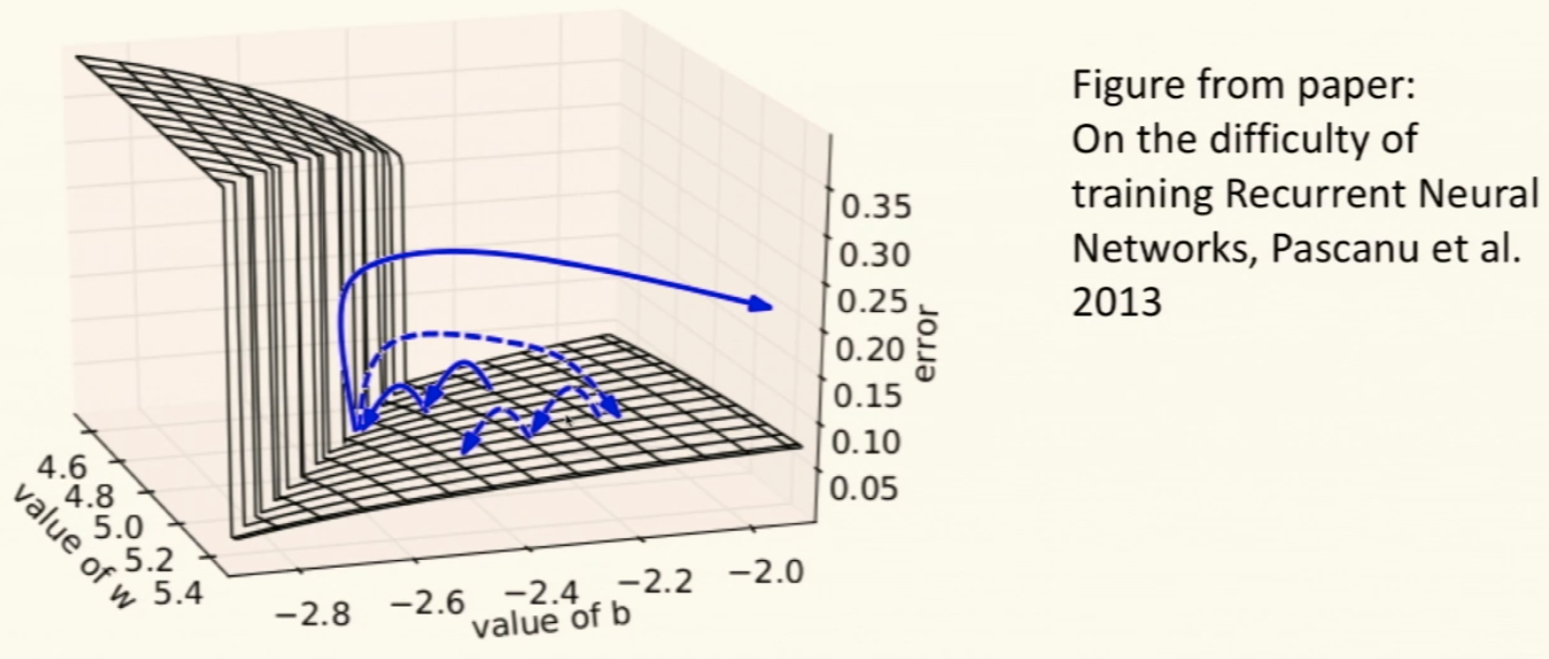
- The image above is that of the Error Surface of a single hidden unit RNN
- The observation here is that there exists High Curvature Walls.
  This Curvature Wall will move the gradient to a very different/far, probably less useful area. Thus, if we clip the gradients we will avoid the walls and will remain in the more useful area that we were exploring already.
  Draw a line between the original point on the Error graph and the End (optimized) point then evaluate the Error on points on that line and look at the changes $\rightarrow$ this shows changes in the curvature.

A natural way to represent discrete variables is to regard the output $\mathbf{o}$ as giving the unnormalized log probabilities of each possible value of the discrete variable. We can then apply the softmax operation as a post-processing step to obtain a vector $\hat{\boldsymbol{y}}$ of normalized probabilities over the output. ↩
for any loss function based on comparing the prediction at time $t$ to the training target at time $t$. ↩
In this way, the network can learn to take into account input conditions (such as those it generates itself in the free-running mode) not seen during training and how to map the state back toward one that will make the network generate proper outputs after a few steps. ↩

Recurrent Neural Networks
Deep Learning Book Ch.10

Table of Contents

Introduction

Recurrent Neural Networks Deep Learning Book Ch.10

Table of Contents

Introduction

Recurrent Neural Networks
Deep Learning Book Ch.10