Gradient-Based Optimization
- Define Gradient Methods:
Gradient Methods are algorithms for solving (optimization) minimization problems of the form:$$\min_{x \in \mathbb{R}^{n}} f(x)$$
by doing local search (~ hill-climbing) with the search directions defined by the gradient of the function at the current point.
- Give examples of Gradient-Based Algorithms:
- Gradient Descent: minimizes arbitrary differentiable functions
- Conjugate Gradient: minimizes sparse linear systems w/ symmetric & PD matrices
- Coordinate Descent: minimizes functions of two variables
- What is Gradient Descent:
GD is a first order, iterative algorithm to minimize an objective function \(J(\theta)\) parametrized by a models parameters \(\theta \in \mathbb{R}^d\) by updating the parameters in the opposite direction of the gradient of the objective function \(\nabla_{\theta} J(\theta)\) w.r.t. to the parameters. -
Explain it intuitively:
1) Local Search from a starting location on a hill
2) Feel around how a small movement/step around your location would change the height of the surrounding hill (is the ground higher or lower)
3) Make the movement/step consistent as a small fixed step along some direction
4) Measure the steepness of the hill at the new location in the chosen direction
5) Do so by Approximating the steepness with some local information
6) Measure the change in steepness from your current point to the new point
6) Find the direction that decreases the steepness the most
\(\iff\)1) Local Search from an initial point \(x_0\) on a function
2) Explore the value of the function at different small nudges around \(x_0\)
3) Make the nudges consistent as a small fixed step \(\delta\) along a normalized direction \(\hat{\boldsymbol{u}}\)
4) Evaluate the function at the new location \(x_0 + \delta \hat{\boldsymbol{u}}\)
5) Do so by Approximating the function w/ first-order information (Taylor expansion)
6) Measure the change in value of the objective \(\Delta f\), from current point to the new point
7) Find the direction \(\hat{\boldsymbol{u}}\) that minimizes the function the most - Give its derivation:
1) Start at \(\boldsymbol{x} = x_0\)
2) We would like to know how would a small change in \(\boldsymbol{x}\), namely \(\Delta \boldsymbol{x}\) would affect the value of the function \(f(x)\). This will allow us to evaluate the function:$$f(\mathbf{x}+\Delta \mathbf{x})$$
to find the direction that makes \(f\) decrease the fastest
3) Let’s set up \(\Delta \boldsymbol{x}\), the change in \(\boldsymbol{x}\), as a fixed step \(\delta\) along some normalized direction \(\hat{\boldsymbol{u}}\):$$\Delta \boldsymbol{x} = \delta \hat{\boldsymbol{u}}$$
4) Evaluate the function at the new location:
$$f(\mathbf{x}+\Delta \mathbf{x}) = f(\mathbf{x}+\delta \hat{\boldsymbol{u}})$$
5) Using the first-order approximation:
$$\begin{aligned} f(\mathbf{x}+\delta \hat{\boldsymbol{u}}) &\approx f({\boldsymbol{x}}_0) + \left(({\boldsymbol{x}}_0 - \delta \hat{\boldsymbol{u}}) - {\boldsymbol{x}}_0 \right)^T \nabla_{\boldsymbol{x}} f({\boldsymbol{x}}_0) \\ &\approx f(x_0) + \delta \hat{\boldsymbol{u}}^T \nabla_x f(x_0) \end{aligned}$$
6) The change in \(f\) is:
$$\begin{aligned} \Delta f &= f(\boldsymbol{x}_ 0 + \Delta \boldsymbol{x}) - f(\boldsymbol{x}_ 0) \\ &= f(\boldsymbol{x}_ 0 + \delta \hat{\boldsymbol{u}}) - f(\boldsymbol{x}_ 0)\\ &= \delta \nabla_x f(\boldsymbol{x}_ 0)^T\hat{\boldsymbol{u}} + \mathcal{O}(\delta^2) \\ &= \delta \nabla_x f(\boldsymbol{x}_ 0)^T\hat{\boldsymbol{u}} \\ &\geq -\delta\|\nabla f(\boldsymbol{x}_ 0)\|_ 2 \end{aligned}$$
where
$$\nabla_x f(\boldsymbol{x}_ 0)^T\hat{\boldsymbol{u}} \in \left[-\|\nabla f(\boldsymbol{x}_ 0)\|_ 2, \|\nabla f(\boldsymbol{x}_ 0)\|_ 2\right]$$
since \(\hat{\boldsymbol{u}}\) is a unit vector; either aligned with \(\nabla_x f(\boldsymbol{x}_ 0)\) or in the opposite direction; it contributes nothing to the magnitude of the dot product.
7) So, the \(\hat{\boldsymbol{u}}\) that changes the above inequality to equality, achieves the largest negative value (moves the most downhill). That vector \(\hat{\boldsymbol{u}}\) is, then, the one in the negative direction of \(\nabla_x f(\boldsymbol{x}_ 0)\); the opposite direction of the gradient.
\(\implies\)$$\hat{\boldsymbol{u}} = - \dfrac{\nabla_x f(x)}{\|\nabla_x f(x)\|_ 2}$$
Finally, The method of steepest/gradient descent proposes a new point to decrease the value of \(f\):
$$\boldsymbol{x}^{\prime}=\boldsymbol{x}-\epsilon \nabla_{\boldsymbol{x}} f(\boldsymbol{x})$$
where \(\epsilon\) is the learning rate, defined as:
$$\epsilon = \dfrac{\delta}{\left\|\nabla_{x} f(x)\right\|_ {2}}$$
- What is the learning rate?
Learning rate is a hyper-parameter that controls how much we are adjusting the weights of our network with respect the loss gradient; defined as:$$\epsilon = \dfrac{\delta}{\left\|\nabla_{x} f(x)\right\|_ {2}}$$
- Where does it come from?
The learning rate comes from a modification of the step-size in the GD derivation.
We get the learning rate by employing a simple idea:
We have a fixed step-size \(\delta\) that dictated how much we should be moving in the direction of steepest descent. However, we would like to keep the step-size from being too small or overshooting. The idea is to make the step-size proportional to the magnitude of the gradient (i.e. some constant multiplied by the magnitude of the gradient):$$\delta = \epsilon \left\|\nabla_{x} f(x)\right\|_ {2}$$
If we do so, we get a nice cancellation as follows:
$$\begin{aligned}\Delta \boldsymbol{x} &= \delta \hat{\boldsymbol{u}} \\ &= -\delta \dfrac{\nabla_x f(x)}{\|\nabla_x f(x)\|_ 2} \\ &= - \epsilon \left\|\nabla_{x} f(x)\right\|_ {2} \dfrac{\nabla_x f(x)}{\|\nabla_x f(x)\|_ 2} \\ &= - \dfrac{\epsilon \left\|\nabla_{x} f(x)\right\|_ {2}}{\|\nabla_x f(x)\|_ 2} \nabla_x f(x) \\ &= - \epsilon \nabla_x f(x) \end{aligned}$$
where now we have a fixed learning rate instead of a fixed step-size.
- How does it relate to the step-size?
[Answer above] - We go from having a fixed step-size to [blank]:
a fixed learning rate.
- What is its range?
\([0.0001, 0.4]\) - How do we choose the learning rate?
- Choose a starting lr from the range \([0.0001, 0.4]\) and adjust using cross-validation (lr is a HP).
- Do
- Set it to a small constant
- Smooth Functions (non-NN):
- Line Search: evaluate \(f\left(\boldsymbol{x}-\epsilon \nabla_{\boldsymbol{x}} f(\boldsymbol{x})\right)\) for several values of \(\epsilon\) and choose the one that results in the smallest objective value.
E.g. Secant Method, Newton-Raphson Method (may need Hessian, hard for large dims) - Trust Region Method
- Line Search: evaluate \(f\left(\boldsymbol{x}-\epsilon \nabla_{\boldsymbol{x}} f(\boldsymbol{x})\right)\) for several values of \(\epsilon\) and choose the one that results in the smallest objective value.
- Non-Smooth Functions (non-NN):
- Direct Line Search
E.g. golden section search
- Direct Line Search
- Grid Search: is simply an exhaustive searching through a manually specified subset of the hyperparameter space of a learning algorithm. It is guided by some performance metric, typically measured by cross-validation on the training set or evaluation on a held-out validation set.
- Population-Based Training (PBT): is an elegant implementation of using a genetic algorithm for hyper-parameter choice.
- Bayesian Optimization: is a global optimization method for noisy black-box functions.
- Use larger lr and use a learning rate schedule
- Compare Line Search vs Trust Region:
Trust-region methods are in some sense dual to line-search methods: trust-region methods first choose a step size (the size of the trust region) and then a step direction, while line-search methods first choose a step direction and then a step size. - Learning Rate Schedule:
- Define:
A learning rate schedule changes the learning rate during learning and is most often changed between epochs/iterations. This is mainly done with two parameters: decay and momentum. - List Types:
- Time-based learning schedules alter the learning rate depending on the learning rate of the previous time iteration. Factoring in the decay the mathematical formula for the learning rate is:
$${\displaystyle \eta_{n+1}={\frac {\eta_{n}}{1+dn}}}$$
where \(\eta\) is the learning rate, \(d\) is a decay parameter and \(n\) is the iteration step.
- Step-based learning schedules changes the learning rate according to some pre defined steps:
$${\displaystyle \eta_{n}=\eta_{0}d^{floor({\frac {1+n}{r}})}}$$
where \({\displaystyle \eta_{n}}\) is the learning rate at iteration \(n\), \(\eta_{0}\) is the initial learning rate, \(d\) is how much the learning rate should change at each drop (0.5 corresponds to a halving) and \(r\) corresponds to the droprate, or how often the rate should be dropped (\(10\) corresponds to a drop every \(10\) iterations). The floor function here drops the value of its input to \(0\) for all values smaller than \(1\).
- Exponential learning schedules are similar to step-based but instead of steps a decreasing exponential function is used. The mathematical formula for factoring in the decay is:
$$ {\displaystyle \eta_{n}=\eta_{0}e^{-dn}}$$
where \(d\) is a decay parameter.
- Time-based learning schedules alter the learning rate depending on the learning rate of the previous time iteration. Factoring in the decay the mathematical formula for the learning rate is:
- Define:
- Where does it come from?
-
Describe the convergence of the algorithm:
Gradient Descent converges when every element of the gradient is zero, or very close to zero within some threshold.With certain assumptions on \(f\) (convex, \(\nabla f\) lipschitz) and particular choices of \(\epsilon\) (chosen via line-search etc.), convergence to a local minimum can be guaranteed.
Moreover, if \(f\) is convex, all local minima are global minimia, so convergence is to the global minimum. - How does GD relate to Euler?
Gradient descent can be viewed as applying Euler’s method for solving ordinary differential equations \({\displaystyle x'(t)=-\nabla f(x(t))}\) to a gradient flow. - List the variants of GD:
- Batch Gradient Descent
- Stochastic GD
- Mini-Batch GD
- How do they differ? Why?:
There are three variants of gradient descent, which differ in the amount of data used to compute the gradient. The amount of data imposes a trade-off between the accuracy of the parameter updates and the time it takes to perform the update.
- BGD:
Batch Gradient Descent AKA Vanilla Gradient Descent, computes the gradient of the objective wrt. the parameters \(\theta\) for the entire dataset:$$\theta=\theta-\epsilon \cdot \nabla_{\theta} J(\theta)$$
- Properties:
- Since we need to compute the gradient for the entire dataset for each update, this approach can be very slow and is intractable for datasets that can’t fit in memory.
- Moreover, batch-GD doesn’t allow for an online learning approach.
- Properties:
- SGD:
SGD performs a parameter update for each data-point:$$\theta=\theta-\epsilon \cdot \nabla_{\theta} J\left(\theta ; x^{(i)} ; y^{(i)}\right)$$
- Properties:
- SGD exhibits a lot of fluctuation and has a lot of variance in the parameter updates. However, although, SGD can potentially move in the wrong direction due to limited information; in-practice, if we slowly decrease the learning-rate, it shows the same convergence behavior as batch gradient descent, almost certainly converging to a local or the global minimum for non-convex and convex optimization respectively.
- Moreover, the fluctuations it exhibits enables it to jump to new and potentially better local minima.
- How should we handle the lr in this case? Why?
We should reduce the lr after every epoch:
This is due to the fact that the random sampling of batches acts as a source of noise which might make SGD keep oscillating around the minima without actually reaching it. - What conditions guarantee convergence of SGD?
The following conditions guarantee convergence under convexity conditions for SGD:
$$\begin{array}{l}{\sum_{k=1}^{\infty} \epsilon_{k}=\infty, \quad \text { and }} \\ {\sum_{k=1}^{\infty} \epsilon_{k}^{2}<\infty}\end{array}$$
- Properties:
- M-BGD:
A hybrid approach that perform updates for a, pre-specified, mini-batch of \(n\) training examples:$$\theta=\theta-\epsilon \cdot \nabla_{\theta} J\left(\theta ; x^{(i : i+n)} ; y^{(i : i+n)}\right)$$
- What advantages does it have?
- Reduce the variance of the parameter updates \(\rightarrow\) more stable convergence
- Makes use of matrix-vector highly optimized libraries
- Computationally efficient compared to stochastic gradient descent.
- Improve generalization by finding flat minima.
- Improving convergence, by using mini-batches we approximating the gradient of the entire training set, which might help to avoid local minima.
- What advantages does it have?
- Explain the different kinds of gradient-descent optimization procedures:
- Batch Gradient Descent AKA Vanilla Gradient Descent, computes the gradient of the objective wrt. the parameters \(\theta\) for the entire dataset:
$$\theta=\theta-\epsilon \cdot \nabla_{\theta} J(\theta)$$
- SGD performs a parameter update for each data-point:
$$\theta=\theta-\epsilon \cdot \nabla_{\theta} J\left(\theta ; x^{(i)} ; y^{(i)}\right)$$
- Mini-batch Gradient Descent a hybrid approach that perform updates for a, pre-specified, mini-batch of \(n\) training examples:
$$\theta=\theta-\epsilon \cdot \nabla_{\theta} J\left(\theta ; x^{(i : i+n)} ; y^{(i : i+n)}\right)$$
- Batch Gradient Descent AKA Vanilla Gradient Descent, computes the gradient of the objective wrt. the parameters \(\theta\) for the entire dataset:
- State the difference between SGD and GD?
Gradient Descent’s cost-function iterates over ALL training samples.
Stochastic Gradient Descent’s cost-function only accounts for ONE training sample, chosen at random. - When would you use GD over SDG, and vice-versa?
GD theoretically minimizes the error function better than SGD. However, SGD converges much faster once the dataset becomes large.
That means GD is preferable for small datasets while SGD is preferable for larger ones.
-
What is the problem of vanilla approaches to GD?
All the variants described above, however, do not guarantee “good” convergence due to some challenges.- List the challenges that account for the problem above:
- Choosing a proper learning rate is usually difficult:
A learning rate that is too small leads to painfully slow convergence, while a learning rate that is too large can hinder convergence and cause the loss function to fluctuate around the minimum or even to diverge. - Inability to adapt to the specific characteristics of the dataset:
Learning rate schedules try to adjust the learning rate during training by e.g. annealing, i.e. reducing the learning rate according to a pre-defined schedule or when the change in objective between epochs falls below a threshold. These schedules and thresholds, however, have to be defined in advance and are thus unable to adapt to a dataset’s characteristics. - The learning rate is fixed for all parameter updates:
If our data is sparse and our features have very different frequencies, we might not want to update all of them to the same extent, but perform a larger update for rarely occurring features. - Another key challenge of minimizing highly non-convex error functions common for neural networks is avoiding getting trapped in their numerous suboptimal local minima. Dauphin et al. argue that the difficulty arises in fact not from local minima but from saddle points, i.e. points where one dimension slopes up and another slopes down. These saddle points are usually surrounded by a plateau of the same error, which makes it notoriously hard for SGD to escape, as the gradient is close to zero in all dimensions.
- Choosing a proper learning rate is usually difficult:
- List the challenges that account for the problem above:
- List the different strategies for optimizing GD:
- Adapt our updates to the slope of our error function
- Adapt our updates to the importance of each individual parameter
- List the different variants for optimizing GD:
- Adapt our updates to the slope of our error function:
- Momentum
- Nesterov Accelerated Gradient
- Adapt our updates to the importance of each individual parameter:
- Adagrad
- Adadelta
- RMSprop
- Adam
- AdaMax
- Nadam
- AMSGrad
- Adapt our updates to the slope of our error function:
- Momentum:
- Motivation:
SGD has trouble navigating ravines (i.e. areas where the surface curves much more steeply in one dimension than in another) which are common around local optima.
In these scenarios, SGD oscillates across the slopes of the ravine while only making hesitant progress along the bottom towards the local optimum. - Definitions/Algorithm:
Momentum is a method that helps accelerate SGD in the relevant direction and dampens oscillations (image^). It does this by adding a fraction \(\gamma\) of the update vector of the past time step to the current update vector:$$\begin{aligned} v_{t} &=\gamma v_{t-1}+\eta \nabla_{\theta} J(\theta) \\ \theta &=\theta-v_{t} \end{aligned}$$
-
Intuition:
Essentially, when using momentum, we push a ball down a hill. The ball accumulates momentum as it rolls downhill, becoming faster and faster on the way (until it reaches its terminal velocity if there is air resistance, i.e. \(\gamma < 1\)). The same thing happens to our parameter updates: The momentum term increases for dimensions whose gradients point in the same directions and reduces updates for dimensions whose gradients change directions. As a result, we gain faster convergence and reduced oscillation.In this case we think of the equation as:
$$v_{t} =\underbrace{\gamma}_{\text{friction }} \: \underbrace{v_{t-1}}_{\text{velocity}}+\eta \underbrace{\nabla_{\theta} J(\theta)}_ {\text{acceleration}}$$
- Parameter Settings:
The momentum term \(\gamma\) is usually set to \(0.9\) or a similar value, and \(v_0 = 0\).
- Motivation:
- Nesterov Accelerated Gradient (Momentum):
- Motivation:
Momentum is good, however, a ball that rolls down a hill, blindly following the slope, is highly unsatisfactory. We’d like to have a smarter ball, a ball that has a notion of where it is going so that it knows to slow down before the hill slopes up again. - Definitions/Algorithm:
NAG is a way to five our momentum term this kind of prescience. Since we know that we will use the momentum term \(\gamma v_{t-1}\) to move the parameters \(\theta\), we can compute a rough approximation of the next position of the parameters with \(\theta - \gamma v_{t-1}\) (w/o the gradient). This allows us to, effectively, look ahead by calculating the gradient not wrt. our current parameters \(\theta\) but wrt. the approximate future position of our parameters:$$\begin{aligned} v_{t} &=\gamma v_{t-1}+\eta \nabla_{\theta} J\left(\theta-\gamma v_{t-1}\right) \\ \theta &=\theta-v_{t} \end{aligned}$$
- Intuition:
While Momentum first computes the current gradient (small blue vector) and then takes a big jump in the direction of the updated accumulated gradient (big blue vector), NAG first makes a big jump in the direction of the previous accumulated gradient (brown vector), measures the gradient and then makes a correction (red vector), which results in the complete NAG update (green vector). This anticipatory update prevents us from going too fast and results in increased responsiveness, which has significantly increased the performance of RNNs on a number of tasks. - Parameter Settings:
\(\gamma = 0.9\), - Successful Applications:
This really helps the optimization of recurrent neural networks
- Motivation:
- Adagrad
- Motivation:
Now that we are able to adapt our updates to the slope of our error function and speed up SGD in turn, we would also like to adapt our updates to each individual parameter to perform larger or smaller updates depending on their importance. - Definitions/Algorithm:
Adagrad is an algorithm for gradient-based optimization that does just this: It adapts the learning rate to the parameters, performing smaller updates (i.e. low learning rates) for parameters associated with frequently occurring features, and larger updates (i.e. high learning rates) for parameters associated with infrequent features. - Intuition:
Adagrad uses a different learning rate for every parameter \(\theta_i\) at every time step \(t\), so, we first show Adagrad’s per-parameter update.
Adagrad per-parameter update:
The SGD update for every parameter \(\theta_i\) at each time step \(t\) is:$$\theta_{t+1, i}=\theta_{t, i}-\eta \cdot g_{t, i}$$
where \(g_{t, i}=\nabla_{\theta} J\left(\theta_{t, i}\right.\) is the partial derivative of the objective function w.r.t. to the parameter \(\theta_i\) at time step \(t\), and \(g_{t}\) is the gradient at time-step \(t\).
In its update rule, Adagrad modifies the general learning rate \(\eta\) at each time step \(t\) for every parameter \(\theta_i\) based on the past gradients that have been computed for \(\theta_i\):
$$\theta_{t+1, i}=\theta_{t, i}-\frac{\eta}{\sqrt{G_{t, i i}+\epsilon}} \cdot g_{t, i}$$
\(G_t \in \mathbb{R}^{d \times d}\) here is a diagonal matrix where each diagonal element \(i, i\) is the sum of the squares of the gradients wrt \(\theta_i\) up to time step \(t\)[^12], while \(\epsilon\) is a smoothing term that avoids division by zero (\(\approx 1e - 8\)).
As \(G_t\) contains the sum of the squares of the past gradients w.r.t. to all parameters \(\theta\) along its diagonal, we can now vectorize our implementation by performing a matrix-vector product \(\odot\) between \(G_t\) and \(g_t\):
$$\theta_{t+1}=\theta_{t}-\frac{\eta}{\sqrt{G_{t}+\epsilon}} \odot g_{t}$$
- Parameter Settings:
For the lr, Most implementations use a default value of \(0.01\) and leave it at that. - Successful Application:
Well-suited for dealing with sparse data (because it adapts the lr of each parameter wrt feature frequency) - Properties:
- Well-suited for dealing with sparse data (because it adapts the lr of each parameter wrt feature frequency)
- Eliminates need for manual tuning of lr:
One of Adagrad’s main benefits is that it eliminates the need to manually tune the learning rate. Most implementations use a default value of \(0.01\) and leave it at that. - Weakness \(\rightarrow\) Accumulation of the squared gradients in the denominator:
Since every added term is positive, the accumulated sum keeps growing during training. This in turn causes the learning rate to shrink and eventually become infinitesimally small, at which point the algorithm is no longer able to acquire additional knowledge. - Without the sqrt, the algorithm performs much worse
- Motivation:
- Adadelta
- Motivation:
Adagrad has a weakness where it suffers from aggressive, monotonically decreasing lr by accumulation of the squared gradients in the denominator. The following algorithm aims to resolve this flow. - Definitions/Algorithm:
- Intuition:
- Parameter Settings:
We set \(\gamma\) to a similar value as the momentum term, around \(0.9\). - Properties:
- Eliminates need for lr completely:
With Adadelta, we do not even need to set a default learning rate, as it has been eliminated from the update rule.
- Eliminates need for lr completely:
- Motivation:
- RMSprop
- Motivation:
RMSprop and Adadelta have both been developed independently around the same time stemming from the need to resolve Adagrad’s radically diminishing learning rates. - Definitions/Algorithm:
RMSprop is an unpublished, adaptive learning rate method proposed by Geoff Hinton in Lecture 6e of his Coursera Class. - Intuition:
RMSprop in fact is identical to the first update vector of Adadelta that we derived above:$$\begin{align} \begin{split} E[g^2]_t &= 0.9 E[g^2]_{t-1} + 0.1 g^2_t \\ \theta_{t+1} &= \theta_{t} - \dfrac{\eta}{\sqrt{E[g^2]_t + \epsilon}} g_{t} \end{split} \end{align}$$
RMSprop as well divides the learning rate by an exponentially decaying average of squared gradients.
- Parameter Settings:
Hinton suggests \(\gamma\) to be set to \(0.9\), while a good default value for the learning rate \(\eta\) is \(0.001\). - Properties:
Works well with RNNs.
- Motivation:
- Adam
- Motivation:
Adding momentum to Adadelta/RMSprop. - Definitions/Algorithm:
Adaptive Moment Estimation (Adam) is another method that computes adaptive learning rates for each parameter. In addition to storing an exponentially decaying average of past squared gradients \(v_t\) like Adadelta and RMSprop, Adam also keeps an exponentially decaying average of past gradients \(m_t\), similar to momentum. - Intuition:
Adam VS Momentum:
Whereas momentum can be seen as a ball running down a slope, Adam behaves like a heavy ball with friction, which thus prefers flat minima in the error surface. - Parameter Settings:
The authors propose default values of \(0.9\) for \(\beta_1\), \(0.999\) for \(\beta_2\), and \(10^{ −8}\) for \(\epsilon\). - Properties:
- They show empirically that Adam works well in practice and compares favorably to other adaptive learning-method algorithms.
- Kingma et al. show that its bias-correction helps Adam slightly outperform RMSprop towards the end of optimization as gradients become sparser. Insofar, Adam might be the best overall choice.
- Motivation:
- Which methods have trouble with saddle points?
SGD, Momentum, and NAG find it difficulty to break symmetry, although the two latter eventually manage to escape the saddle point, while Adagrad, RMSprop, and Adadelta quickly head down the negative slope. - How should you choose your optimizer?
- As we can see, the adaptive learning-rate methods, i.e. Adagrad, Adadelta, RMSprop, and Adam are most suitable and provide the best convergence for these scenarios.
- Sparse Input Data:
If your input data is sparse, then you likely achieve the best results using one of the adaptive learning-rate methods. An additional benefit is that you won’t need to tune the learning rate but likely achieve the best results with the default value.
- Summarize the different variants listed above. How do they compare to each other?
In summary, RMSprop is an extension of Adagrad that deals with its radically diminishing learning rates. It is identical to Adadelta, except that Adadelta uses the RMS of parameter updates in the numerator update rule. Adam, finally, adds bias-correction and momentum to RMSprop. Insofar, RMSprop, Adadelta, and Adam are very similar algorithms that do well in similar circumstances. - What’s a common choice in many research papers?
Interestingly, many recent papers use vanilla SGD without momentum and a simple learning rate annealing schedule. - List additional strategies for optimizing SGD:
- Shuffling and Curriculum Learning
- Batch Normalization
- Early Stopping
- Gradient Noise
Maximum Margin Classifiers
- Define Margin Classifiers:
A margin classifier is a classifier which is able to give an associated distance from the decision boundary for each example. - What is a Margin for a linear classifier?
The margin of a linear classifier is the distance from the decision boundary to the nearest sample point. -
Give the motivation for margin classifiers:
Non-margin classifiers (e.g. Centroid, Perceptron, LR) will converge to a correct classifier on linearly separable data; however, the classifier they converge to is not unique nor the best. - Define the notion of the “best” possible classifier
We assume that if we can maximize the distance between the data points to be classified and the hyperplane that classifies them, then we have reached a boundary that allows for the “best-fit”, i.e. allows for the most room for error. - How can we achieve the “best” classifier?
We enforce a constraint that achieves a classifier that has a maximum-margin. - What unique vector is orthogonal to the hp? Prove it:
The weight vector \(\mathbf{w}\) is orthogonal to the separating-plane/decision-boundary, defined by \(\mathbf{w}^T\mathbf{x} + b = 0\), in the \(\mathcal{X}\) space; Reason:
Since if you take any two points \(\mathbf{x}^\prime\) and \(\mathbf{x}^{\prime \prime}\) on the plane, and create the vector \(\left(\mathbf{x}^{\prime}-\mathbf{x}^{\prime \prime}\right)\) parallel to the plane by subtracting the two points, then the following equations must hold:$$\mathbf{w}^{\top} \mathbf{x}^{\prime}+b=0 \wedge \mathbf{w}^{\top} \mathbf{x}^{\prime \prime}+b=0 \implies \mathbf{w}^{\top}\left(\mathbf{x}^{\prime}-\mathbf{x}^{\prime \prime}\right)=0$$
- What do we mean by “signed distance”? Derive its formula:
The signed distance is the minimum distance from a point to a hyperplane. We solve for the signed distance to achieve the following formula for it: \(d = \dfrac{\| w \cdot x_0 + b \|}{\|w\|},\)
where we have an n-dimensional hyperplane: \(w \cdot x + b = 0\) and a point \(\mathbf{x}_ n\).
Derivation:- Suppose we have an affine hyperplane defined by \(w \cdot x + b\) and a point \(\mathbf{x}_ n\).
- Suppose that \(\mathbf{x} \in \mathbf{R}^n\) is a point satisfying \(w \cdot \mathbf{x} + b = 0\), i.e. it is a point on the plane.
- We construct the vector \(\mathbf{x}_ n−\mathbf{x}\) which points from \(\mathbf{x}\) to \(\mathbf{x}_ n\), and then, project (scalar projection==signed distance) it onto the unique vector perpendicular to the plane, i.e. \(w\),
$$d=| \text{comp}_{w} (\mathbf{x}_ n-\mathbf{x})| = \left| \frac{(\mathbf{x}_ n-\mathbf{x})\cdot w}{\|w\|} \right| = \frac{|\mathbf{x}_ n \cdot w - \mathbf{x} \cdot w|}{\|w\|}.$$
- Since \(\mathbf{x}\) is a vector on the plane, it must satisfy \(w\cdot \mathbf{x}=-b\) so we get
$$d=| \text{comp}_{w} (\mathbf{x}_ n-\mathbf{x})| = \frac{|\mathbf{x}_ n \cdot w +b|}{\|w\|}$$
Thus, we conclude that if \(\|w\| = 1\) then the signed distance from a datapoint \(X_i\) to the hyperplane is \(\|wX_i + b\|\).
- Given the formula for signed distance, calculate the “distance of the point closest to the hyperplane”:
Let \(X_n\) be the point that is closest to the plane, and let \(\hat{w} = \dfrac{w}{\|w\|}\).
Take any point \(X\) on the plane, and let \(\vec{v}\) be the vector \(\vec{v} = X_n - X\).
Now, the distance, \(d\) is equal to$$\begin{align} d & \ = \vert\hat{w}^{\top}\vec{v}\vert \\ & \ = \vert\hat{w}^{\top}(X_n - X)\vert \\ & \ = \vert\hat{w}^{\top}X_n - \hat{w}^{\top}X)\vert \\ & \ = \dfrac{1}{\|w\|}\vert w^{\top}X_n + b - w^{\top}X) - b\vert , & \text{we add and subtract the bias } b\\ & \ = \dfrac{1}{\|w\|}\vert (w^{\top}X_n + b) - (w^{\top}X + b)\vert \\ & \ = \dfrac{1}{\|w\|}\vert (w^{\top}X_n + b) - (0)\vert , & \text{from the eq. of the plane on a point on the plane} \\ & \ = \dfrac{\vert (w^{\top}X_n + b)\vert}{\|w\|} \end{align} $$
- Use geometric properties of the hp to Simplify the expression for the distance of the closest point to the hp, above
First, we notice that for any given plane \(w^Tx = 0\), the equations, \(\gamma * w^Tx = 0\), where \(\gamma \in \mathbf{R}\) is a scalar, basically characterize the same plane and not many planes.
This is because \(w^Tx = 0 \iff \gamma * w^Tx = \gamma * 0 \iff \gamma * w^Tx = 0\).
The above implies that any model that takes input \(w\) and produces a margin, will have to be Scale Invariant.
To get around this and simplify the analysis, I am going to consider all the representations of the same plane, and I am going to pick one where we normalize (re-scale) the weight \(w\) such that the signed distance (distance to the point closest to the margin) is equal to one:$$|w^Tx_n| > 0 \rightarrow |w^Tx_n| = 1$$
, where \(x_n\) is the point closest to the plane.
We constraint the hyperplane by normalizing \(w\) to this equation \(|w^Tx_i| = 1\) or with added bias, \(|w^Tx_i + b| = 1\).
\(\implies\)$$\begin{align} d & \ = \dfrac{\vert (w^{\top}X_n + b)\vert}{\|w\|} \\ & \ = \dfrac{\vert (1)\vert}{\|w\|} , & \text{from the constraint on the distance of the closest point} \\ & \ = \dfrac{1}{\|w\|} \end{align} $$
- Characterize the margin, mathematically:
we can characterize the margin, with its size, as the distance, \(\frac{1}{\|\mathbf{w}\|}\), between the hyperplane/boundary and the closest point to the plane \(\mathbf{x}_ n\), in both directions (multiply by 2) \(= \frac{2}{\|\mathbf{w}\|}\) ; given the condition we specified earlier \(\left|\mathbf{w}^{\top} \mathbf{x}_ {n} + b\right|=1\) for the closest point \(\mathbf{x}_ n\). - Characterize the “Slab Existence”:
The analysis done above allows us to conclusively prove that there exists a slab of width \(\dfrac{2}{\|w\|}\) containing no sample points where the hyperplane runs through (bisects) its center. - Formulate the optimization problem of maximizing the margin wrt analysis above:
We formulate the optimization problem of maximizing the margin by maximizing the distance, subject to the condition on how we derived the distance:$$\max_{\mathbf{w}} \dfrac{2}{\|\mathbf{w}\|} \:\:\: : \:\: \min _{n=1,2, \ldots, N}\left|\mathbf{w}^{\top} \mathbf{x}_{n}+b\right|=1$$
- Reformulate the optimization problem above to a more “friendly” version (wrt optimization -> put in standard form):
We can reformulate by (1) Flipping and Minimizing, (2) Taking a square since it’s monotonic and convex, and (3) noticing that \(\left|\mathbf{w}^{T} \mathbf{x}_ {n}+b\right|=y_{n}\left(\mathbf{w}^{T} \mathbf{x}_ {n}+b\right)\) (since the signal and label must agree, their product will always be positive) and the \(\min\) operator can be replaced by ensuring that for all the points the condition \(y_{n}\left(\mathbf{w}^{\top} \mathbf{x}_ {n}+b\right) \geq 1\) holds proof (by contradiction) as:$$\min_w \dfrac{1}{2} \mathbf{w}^T\mathbf{w} \:\:\: : \:\: y_{n}\left(\mathbf{w}^{\top} \mathbf{x}_ {n}+b\right) \geq 1 \:\: \forall i \in [1,N]$$
Now when we solve the “friendly” equation above, we will get the separating plane with the best possible margin (best=biggest).
- Give the final (standard) formulation of the “Optimization problem for maximum margin classifiers”:
$$\min_w \dfrac{1}{2} \mathbf{w}^T\mathbf{w} \:\:\: : \:\: y_{n}\left(\mathbf{w}^{\top} \mathbf{x}_ {n}+b\right) \geq 1 \:\: \forall i \in [1,N]$$
- What kind of formulation is it (wrt optimization)? What are the parameters?
The above problem is a Quadratic Program, in \(d + 1\)-dimensions and \(n\)-constraints, in standard form.
- Give the final (standard) formulation of the “Optimization problem for maximum margin classifiers”:
Hard-Margin SVMs
- Define:
- SVMs:
1.*Support Vector Machines** (SVMs) are supervised learning models with associated learning algorithms that analyze data used for classification and regression analysis.
The SVM is a Maximum Margin Classifier that aims to find the “maximum-margin hyperplane” that divides the group of points \({\displaystyle {\vec {x}}_{i}} {\vec {x}}_{i}\) for which \({\displaystyle y_{i}=1}\) from the group of points for which \({\displaystyle y_{i}=-1}\). - Support Vectors:
1.*Support Vectors** are the data-points that lie exactly on the margin (i.e. on the boundary of the slab).
They satisfy \(\|w^TX' + b\| = 1, \forall\) support vectors \(X'\) - Hard-Margin SVM:
The Hard-Margin SVM is just a maximum-margin classifier with features and kernels (discussed later).
- SVMs:
- Define the following wrt hard-margin SVM:
- Goal:
Find weights ‘\(w\)’ and scalar ‘\(b\)’ that correctly classifies the data-points and, moreover, does so in the “best” possible way. - Procedure:
(1) Use a linear classifier (2) But, Maximize the Margin (3) Do so by Minimizing \(\|w\|\) - Decision Function:
$${\displaystyle f(x)={\begin{cases}1&{\text{if }}\ w\cdot X_i+\alpha>0\\0&{\text{otherwise}}\end{cases}}}$$
- Constraints:
$$y_i(wX_i + b) \geq 1, \forall i \in [1,n]$$
- The Optimization Problem:
Find weights ‘\(w\)’ and scalar ‘\(b\)’ that minimize$$ \dfrac{1}{2} w^Tw$$
Subject to
$$y_i(wX_i + b) \geq 1, \forall i \in [1,n]$$
Formally,
$$\min_w \dfrac{1}{2}w^Tw \:\:\: : \:\: y_i(wX_i + b) \geq 1, \forall i \in [1,n]$$
- The Optimization Method:
The SVM optimization problem reduces to a Quadratic Program.
- Goal:
- Elaborate on the generalization analysis:
We notice that, geometrically, the hyperplane (the maximum margin classifier) is completely characterized by the support vectors (the vectors that lie on the margin).
A very important conclusion arises.
The maximum margin classifier (SVM) depends only on the number of support vectors and not on the dimension of the problem.
This implies that the computation doesn’t scale up with the dimension and, also implies, that the kernel trick works very well. - List the properties:
- In addition to performing linear classification, SVMs can efficiently perform a non-linear classification using what is called the kernel trick, implicitly mapping their inputs into high-dimensional feature spaces.
- The hyperplane is determined solely by its support vectors.
- The SVM always converges on linearly separable data.
- The Hard-Margin SVM fails if the data is not linearly separable.
- The Hard-Margin SVM is quite sensitive to outliers
- Give the solution to the optimization problem for H-M SVM:
To solve the above problem, we need something that deals with inequality constraints; thus, we use the KKT method for solving a Lagrnagian under inequality constraints.
The Lagrange Formulation:- Formulate the Lagrangian:
- Take each inequality constraint and put them in the zero-form (equality with Zero)
- Multiply each inequality by a Lagrange Multiplier \(\alpha_n\)
- Add them to the objective function \(\min_w \dfrac{1}{2} \mathbf{w}^T\mathbf{w}\)
The sign will be \(-\) (negative) simply because the inequality is \(\geq 0\)
$$\min_{w, b} \max_{\alpha_n} \mathcal{L}(\mathbf{w}, b, \boldsymbol{\alpha}) = \dfrac{1}{2} \mathbf{w}^T\mathbf{w} -\sum_{n=1}^{N} \alpha_{n}\left(y_{n}\left(\mathbf{w}^{\top} \mathbf{x}_ {n}+b\right)-1\right) \:\:\: : \:\: \alpha_n \geq 0$$
- Optimize the objective independently, for each of the unconstrained variables:
- Gradient w.r.t. \(\mathbf{w}\):
$$\nabla_{\mathrm{w}} \mathcal{L}=\mathrm{w}-\sum_{n=1}^{N} \alpha_{n} y_{n} \mathrm{x}_ {n}=0 \\ \implies \\ \mathbf{w}=\sum_{n=1}^{N} \alpha_{n} y_{n} \mathbf{x}_ {n}$$
- Derivative w.r.t. \(b\):
$$\frac{\partial \mathcal{L}}{\partial b}=-\sum_{n=1}^{N} \alpha_{n} y_{n}=0 \\ \implies \\ \sum_{n=1}^{N} \alpha_{n} y_{n}=0$$
- Gradient w.r.t. \(\mathbf{w}\):
- Get the Dual Formulation w.r.t. the (tricky) constrained variable \(\alpha_n\):
- Substitute with the above conditions in the original lagrangian (such that the optimization w.r.t. \(\alpha_n\) will become free of \(\mathbf{w}\) and \(b\):
$$\mathcal{L}(\boldsymbol{\alpha})=\sum_{n=1}^{N} \alpha_{n}-\frac{1}{2} \sum_{n=1}^{N} \sum_{m=1}^{N} y_{n} y_{m} \alpha_{n} \alpha_{m} \mathbf{x}_{n}^{\mathrm{T}} \mathbf{x}_{m}$$
- Notice that the first constraint \(\mathbf{w}=\sum_{n=1}^{N} \alpha_{n} y_{n} \mathbf{x}_ {n}\) has-no-effect/doesn’t-constraint \(\alpha_n\) so it’s a vacuous constraint. However, not the second constraint \(\sum_{n=1}^{N} \alpha_{n} y_{n}=0\).
- Set the optimization objective and the constraints, a quadratic function in \(\alpha_n\):
$$\max_{\alpha} \mathcal{L}(\boldsymbol{\alpha})=\sum_{n=1}^{N} \alpha_{n}-\frac{1}{2} \sum_{n=1}^{N} \sum_{m=1}^{N} y_{n} y_{m} \alpha_{n} \alpha_{m} \mathbf{x}_{n}^{\mathrm{T}} \mathbf{x}_{m} \\ \:\:\:\:\:\:\:\:\:\: : \:\: \alpha_n \geq 0 \:\: \forall \: n= 1, \ldots, N \:\: \wedge \:\: \sum_{n=1}^{N} \alpha_{n} y_{n}=0$$
- Substitute with the above conditions in the original lagrangian (such that the optimization w.r.t. \(\alpha_n\) will become free of \(\mathbf{w}\) and \(b\):
- Set the problem as a Quadratic Programming problem:
- Change the maximization to minimization by flipping the signs:
$$\min _{\alpha} \frac{1}{2} \sum_{n=1}^{N} \sum_{m=1}^{N} y_{n} y_{m} \alpha_{n} \alpha_{m} \mathbf{x}_{0}^{\mathrm{T}} \mathbf{x}_{m}-\sum_{n=1}^{N} \alpha_{n}$$
- Isolate the Coefficients from the \(\alpha_n\)s and set in matrix-form:
$$\min _{\alpha} \frac{1}{2} \alpha^{\top} \underbrace{\begin{bmatrix} y_{1} y_{1} \mathbf{x}_{1}^{\top} \mathbf{x}_{1} & y_{1} y_{2} \mathbf{x}_{1}^{\top} \mathbf{x}_{2} & \ldots & y_{1} y_{N} \mathbf{x}_{1}^{\top} \mathbf{x}_{N} \\ y_{2} y_{1} \mathbf{x}_{2}^{\top} \mathbf{x}_{1} & y_{2} y_{2} \mathbf{x}_{2}^{\top} \mathbf{x}_{2} & \ldots & y_{2} y_{N} \mathbf{x}_{2}^{\top} \mathbf{x}_{N} \\ \ldots & \ldots & \ldots & \ldots \\ y_{N} y_{1} \mathbf{x}_{N}^{\top} \mathbf{x}_{1} & y_{N} y_{2} \mathbf{x}_{N}^{\top} \mathbf{x}_{2} & \ldots & y_{N} y_{N} \mathbf{x}_{N}^{\top} \mathbf{x}_{N} \end{bmatrix}}_{\text{quadratic coefficients}} \alpha+\underbrace{\left(-1^{\top}\right)}_ {\text {linear }} \alpha \\ \:\:\:\:\:\:\:\:\:\: : \:\: \underbrace{\mathbf{y}^{\top} \boldsymbol{\alpha}=0}_{\text {linear constraint }} \:\: \wedge \:\: \underbrace{0}_{\text {lower bounds }} \leq \alpha \leq \underbrace{\infty}_{\text {upper bounds }} $$
The Quadratic Programming Package asks you for the Quadratic Term (Matrix) and the Linear Term, and for the Linear Constraint and the Range of \(\alpha_n\)s; and then, gives you back an \(\mathbf{\alpha}\).
Equivalently:
$$\min _{\alpha} \frac{1}{2} \boldsymbol{\alpha}^{\mathrm{T}} \mathrm{Q} \boldsymbol{\alpha}-\mathbf{1}^{\mathrm{T}} \boldsymbol{\alpha} \quad \text {subject to } \quad \mathbf{y}^{\mathrm{T}} \boldsymbol{\alpha}=0 ; \quad \boldsymbol{\alpha} \geq \mathbf{0}$$
- Change the maximization to minimization by flipping the signs:
- What method does it require to be solved:
To solve the above problem, we need something that deals with inequality constraints; thus, we use the KKT method for solving a Lagrnagian under inequality constraints. - Formulate the Lagrangian:
- Take each inequality constraint and put them in the zero-form (equality with Zero)
- Multiply each inequality by a Lagrange Multiplier \(\alpha_n\)
- Add them to the objective function \(\min_w \dfrac{1}{2} \mathbf{w}^T\mathbf{w}\)
The sign will be \(-\) (negative) simply because the inequality is \(\geq 0\)
$$\min_{w, b} \max_{\alpha_n} \mathcal{L}(\mathbf{w}, b, \boldsymbol{\alpha}) = \dfrac{1}{2} \mathbf{w}^T\mathbf{w} -\sum_{n=1}^{N} \alpha_{n}\left(y_{n}\left(\mathbf{w}^{\top} \mathbf{x}_ {n}+b\right)-1\right) \:\:\: : \:\: \alpha_n \geq 0$$
- Optimize the objective for each variable:
- Gradient w.r.t. \(\mathbf{w}\):
$$\nabla_{\mathrm{w}} \mathcal{L}=\mathrm{w}-\sum_{n=1}^{N} \alpha_{n} y_{n} \mathrm{x}_ {n}=0 \\ \implies \\ \mathbf{w}=\sum_{n=1}^{N} \alpha_{n} y_{n} \mathbf{x}_ {n}$$
- Derivative w.r.t. \(b\):
$$\frac{\partial \mathcal{L}}{\partial b}=-\sum_{n=1}^{N} \alpha_{n} y_{n}=0 \\ \implies \\ \sum_{n=1}^{N} \alpha_{n} y_{n}=0$$
- Gradient w.r.t. \(\mathbf{w}\):
- Get the Dual Formulation w.r.t. the (tricky) constrained variable \(\alpha_n\):
- Substitute with the above conditions in the original lagrangian (such that the optimization w.r.t. \(\alpha_n\) will become free of \(\mathbf{w}\) and \(b\):
$$\mathcal{L}(\boldsymbol{\alpha})=\sum_{n=1}^{N} \alpha_{n}-\frac{1}{2} \sum_{n=1}^{N} \sum_{m=1}^{N} y_{n} y_{m} \alpha_{n} \alpha_{m} \mathbf{x}_{n}^{\mathrm{T}} \mathbf{x}_{m}$$
- Notice that the first constraint \(\mathbf{w}=\sum_{n=1}^{N} \alpha_{n} y_{n} \mathbf{x}_ {n}\) has-no-effect/doesn’t-constraint \(\alpha_n\) so it’s a vacuous constraint. However, not the second constraint \(\sum_{n=1}^{N} \alpha_{n} y_{n}=0\).
- Set the optimization objective and the constraints, a quadratic function in \(\alpha_n\):
$$\max_{\alpha} \mathcal{L}(\boldsymbol{\alpha})=\sum_{n=1}^{N} \alpha_{n}-\frac{1}{2} \sum_{n=1}^{N} \sum_{m=1}^{N} y_{n} y_{m} \alpha_{n} \alpha_{m} \mathbf{x}_{n}^{\mathrm{T}} \mathbf{x}_{m} \\ \:\:\:\:\:\:\:\:\:\: : \:\: \alpha_n \geq 0 \:\: \forall \: n= 1, \ldots, N \:\: \wedge \:\: \sum_{n=1}^{N} \alpha_{n} y_{n}=0$$
- Substitute with the above conditions in the original lagrangian (such that the optimization w.r.t. \(\alpha_n\) will become free of \(\mathbf{w}\) and \(b\):
- Set the problem as a Quadratic Programming problem:
- Change the maximization to minimization by flipping the signs:
$$\min _{\alpha} \frac{1}{2} \sum_{n=1}^{N} \sum_{m=1}^{N} y_{n} y_{m} \alpha_{n} \alpha_{m} \mathbf{x}_{0}^{\mathrm{T}} \mathbf{x}_{m}-\sum_{n=1}^{N} \alpha_{n}$$
- Isolate the Coefficients from the \(\alpha_n\)s and set in matrix-form:
$$\min _{\alpha} \frac{1}{2} \alpha^{\top} \underbrace{\begin{bmatrix} y_{1} y_{1} \mathbf{x}_{1}^{\top} \mathbf{x}_{1} & y_{1} y_{2} \mathbf{x}_{1}^{\top} \mathbf{x}_{2} & \ldots & y_{1} y_{N} \mathbf{x}_{1}^{\top} \mathbf{x}_{N} \\ y_{2} y_{1} \mathbf{x}_{2}^{\top} \mathbf{x}_{1} & y_{2} y_{2} \mathbf{x}_{2}^{\top} \mathbf{x}_{2} & \ldots & y_{2} y_{N} \mathbf{x}_{2}^{\top} \mathbf{x}_{N} \\ \ldots & \ldots & \ldots & \ldots \\ y_{N} y_{1} \mathbf{x}_{N}^{\top} \mathbf{x}_{1} & y_{N} y_{2} \mathbf{x}_{N}^{\top} \mathbf{x}_{2} & \ldots & y_{N} y_{N} \mathbf{x}_{N}^{\top} \mathbf{x}_{N} \end{bmatrix}}_{\text{quadratic coefficients}} \alpha+\underbrace{\left(-1^{\top}\right)}_ {\text {linear }} \alpha \\ \:\:\:\:\:\:\:\:\:\: : \:\: \underbrace{\mathbf{y}^{\top} \boldsymbol{\alpha}=0}_{\text {linear constraint }} \:\: \wedge \:\: \underbrace{0}_{\text {lower bounds }} \leq \alpha \leq \underbrace{\infty}_ {\text {upper bounds }} $$
- Change the maximization to minimization by flipping the signs:
- What are the inputs and outputs to the Quadratic Program Package?
The Quadratic Programming Package asks you for the Quadratic Term (Matrix) and the Linear Term, and for the Linear Constraint and the Range of \(\alpha_n\)s; and then, gives you back an \(\mathbf{\alpha}\). - Give the final form of the optimization problem in standard form:
$$\min_{\alpha} \frac{1}{2} \boldsymbol{\alpha}^{\mathrm{T}} \mathrm{Q} \boldsymbol{\alpha}-\mathbf{1}^{\mathrm{T}} \boldsymbol{\alpha} \quad \text {subject to } \quad \mathbf{y}^{\mathrm{T}} \boldsymbol{\alpha}=0 ; \quad \boldsymbol{\alpha} \geq \mathbf{0}$$
- Formulate the Lagrangian:
Soft-Margin SVM
- Motivate the soft-margin SVM:
The Hard-Margin SVM faces a few issues:- The Hard-Margin SVM fails if the data is not linearly separable.
- The Hard-Margin SVM is quite sensitive to outliers
The Soft-Margin SVM aims to fix/reconcile these problems.
- What is the main idea behind it?
Allow some points to violate the margin, by introducing slack variables. - Define the following wrt soft-margin SVM:
- Goal:
Find weights ‘\(w\)’ and scalar ‘\(b\)’ that correctly classifies the data-points and, moreover, does so in the “best” possible way, but allow some points to violate the margin, by introducing slack variables. - Procedure:
(1) Use a linear classifier
(2) But, Maximize the Margin
(3) Do so by Minimizing \(\|w\|\)
(4) But allow some points to penetrate the margin - Decision Function:
- Constraints:
$$y_i(wX_i + b) \geq 1 - \zeta_i, \forall i \in [1,n]$$
where the \(\zeta_i\)s are slack variables.
We, also, enforce the non-negativity constraint on the slack variables:$$\zeta_i \geq 0, \:\:\: \forall i \in [1, n]$$
- Why is there a non-negativity constraint?
The non-negativity constraint forces the slack variables to be zero for all points that do not violate the original constraint:
i.e. are not inside the slab.
- Why is there a non-negativity constraint?
- Objective/Cost Function:
$$ R(w) = \dfrac{1}{2} w^Tw + C \sum_{i=1}^n \zeta_i$$
- The Optimization Problem:
Find weights ‘\(w\)’, scalar ‘\(b\)’, and \(\zeta_i\)s that minimize$$ \dfrac{1}{2} w^Tw + C \sum_{i=1}^n \zeta_i$$
Subject to
$$y_i(wX_i + b) \geq 1 - \zeta_i, \zeta_i \geq 0, \forall i \in [1,n]$$
Formally,
$$\min_w \dfrac{1}{2}w^Tw \:\:\: : \:\: y_i(wX_i + b) \geq 1 - \zeta_i, \:\: \zeta_i \geq 0, \forall i \in [1,n]$$
- The Optimization Method:
The SVM optimization problem reduces to a Quadratic Program in \(d + n + 1\)-dimensions and \(2n\)-constraints. - Properties:
- The Soft-Margin SVM will converge on non-linearly separable data.
- Goal:
-
Specify the effects of the regularization hyperparameter \(C\):
Small C Large C Desire Maximizing Margin = \(\dfrac{1}{|w|}\) keep most slack variables zero or small Danger underfitting (High Misclassification) overfitting (awesome training, awful test) outliers less sensitive very sensitive boundary more “flat” more sinuous - Describe the effect wrt over/under fitting:
Increase \(C\) hparam in SVM = causes overfitting
- Describe the effect wrt over/under fitting:
- How do we choose \(C\)?
We choose ‘\(C\)’ with cross-validation. - Give an equivalent formulation in the standard form objective for function estimation (what should it minimize?)
In function estimation we prefer the standard-form objective to minimize (and trade-off); the loss + penalty form.
We introduce a loss function to moderate the use of the slack variables (i.e. to avoid abusing the slack variables), namely, Hinge Loss:$${\displaystyle \max \left(0, 1-y_{i}({\vec {w}}\cdot {\vec {x}}_ {i}-b)\right)}$$
The motivation: We motivate it by comparing it to the traditional \(0-1\) Loss function.
Notice that the \(0-1\) loss is actually non-convex. It has an infinite slope at \(0\). On the other hand, the hinge loss is actually convex.Analysis wrt maximum margin:
This function is zero if the constraint, \(y_{i}({\vec {w}}\cdot {\vec {x}}_ {i}-b)\geq 1\), is satisfied, in other words, if \({\displaystyle {\vec {x}}_{i}} {\vec {x}}_{i}\) lies on the correct side of the margin.
For data on the wrong side of the margin, the function’s value is proportional to the distance from the margin.Modified Objective Function:
$$R(w) = \dfrac{\lambda}{2} w^Tw + \sum_{i=1}^n {\displaystyle \max \left(0, 1-y_{i}({\vec {w}}\cdot {\vec {x}}_ {i}-b)\right)}$$
Proof of equivalence:
$$\begin{align} y_if\left(x_i\right) & \ \geq 1-\zeta_i, & \text{from 1st constraint } \\ \implies \zeta_i & \ \geq 1-y_if\left(x_i\right) \\ \zeta_i & \ \geq 1-y_if\left(x_i\right) \geq 0, & \text{from 2nd positivity constraint on} \zeta_i \\ \iff \zeta_i & \ \geq \max \{0, 1-y_if\left(x_i\right)\} \\ \zeta_i & \ = \max \{0, 1-y_if\left(x_i\right)\}, & \text{minimizing means } \zeta_i \text{reach lower bound}\\ \implies R(w) & \ = \dfrac{\lambda}{2} w^Tw + \sum_{i=1}^n {\displaystyle \max \left(0, 1-y_{i}({\vec {w}}\cdot {\vec {x}}_ {i}-b)\right)}, & \text{plugging in and multplying } \lambda = \dfrac{1}{C} \end{align}$$
The (reformulated) Optimization Problem:
$$\min_{w, b}\dfrac{\lambda}{2} w^Tw + \sum_{i=1}^n {\displaystyle \max \left(0, 1-y_{i}({\vec {w}}\cdot {\vec {x}}_ {i}-b)\right)}$$
Loss Functions
- Define:
-
Loss Functions - Abstractly and Mathematically:
Abstractly, a loss function or cost function is a function that maps an event or values of one or more variables onto a real number, intuitively, representing some “cost” associated with the event.Formally, a loss function is a function \(L :(\hat{y}, y) \in \mathbb{R} \times Y \longmapsto L(\hat{y}, y) \in \mathbb{R}\) that takes as inputs the predicted value \(\hat{y}\) corresponding to the real data value \(y\) and outputs how different they are.
- Distance-Based Loss Functions:
A Loss function \(L(\hat{y}, y)\) is called distance-based if it:- Only depends on the residual:
$$L(\hat{y}, y) = \psi(y-\hat{y}) \:\: \text{for some } \psi : \mathbb{R} \longmapsto \mathbb{R}$$
- Loss is \(0\) when residual is \(0\):
$$\psi(0) = 0$$
- Describe an important property of dist-based losses:
Translation Invariance:
Distance-based losses are translation-invariant:$$L(\hat{y}+a, y+a) = L(\hat{y}, y)$$
- What are they used for?
Regression.
- Only depends on the residual:
- Relative Error - What does it lack?
Relative-Error \(\dfrac{\hat{y}-y}{y}\) is a more natural loss but it is NOT translation-invariant.
-
- List 3 Regression Loss Functions
- MSE
- MAE
- Huber
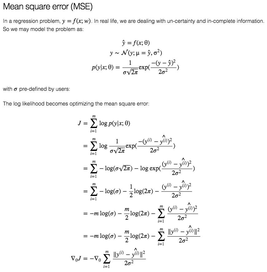
- MSE
- What does it minimize:
The MSE minimizes the sum of squared differences between the predicted values and the target values. - Formula:
$$L(\hat{y}, y) = \dfrac{1}{n} \sum_{i=1}^{n}\left(y_{i}-\hat{y}_ {i}\right)^{2}$$
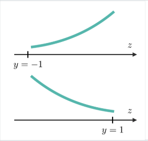
- Graph:
- Derivation:
- What does it minimize:
- MAE
- What does it minimize:
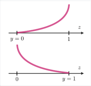
The MAE minimizes the sum of absolute differences between the predicted values and the target values. - Formula:
$$L(\hat{y}, y) = \dfrac{1}{n} \sum_{i=1}^{n}\vert y_{i}-\hat{y}_ {i}\vert$$
- Graph:
- Derivation:
- List properties:
- Solution may be Non-unique
- Robustness to outliers
- Unstable Solutions:
The instability property of the method of least absolute deviations means that, for a small horizontal adjustment of a datum, the regression line may jump a large amount. The method has continuous solutions for some data configurations; however, by moving a datum a small amount, one could “jump past” a configuration which has multiple solutions that span a region. After passing this region of solutions, the least absolute deviations line has a slope that may differ greatly from that of the previous line. In contrast, the least squares solutions is stable in that, for any small adjustment of a data point, the regression line will always move only slightly; that is, the regression parameters are continuous functions of the data. - Data-points “Latching” ref:
- Unique Solution:
If there are \(k\) features (including the constant), then at least one optimal regression surface will pass through \(k\) of the data points; unless there are multiple solutions. - Multiple Solutions:
The region of valid least absolute deviations solutions will be bounded by at least \(k\) lines, each of which passes through at least \(k\) data points.
- Unique Solution:
- What does it minimize:
- Huber Loss
- AKA:
Smooth Mean Absolute Error - Formula:
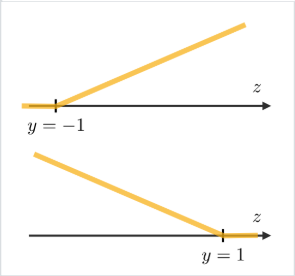
$$L(\hat{y}, y) = \left\{\begin{array}{cc}{\frac{1}{2}(y-\hat{y})^{2}} & {\text {if }|(y-\hat{y})|<\delta} \\ {\delta \vert y-\hat{y}\vert-\frac{1}{2} \delta^2} & {\text {otherwise }}\end{array}\right.$$
- Graph:
- List properties:
- It’s less sensitive to outliers than the MSE as it treats error as square only inside an interval.
- AKA:
-
Analyze MSE vs MAE ref:
MSE MAE Sensitive to outliers Robust to outliers Differentiable Everywhere Non-Differentiable at \(0\) Stable Solutions Unstable Solutions Unique Solution Possibly multiple solutions - Statistical Efficiency:
- “For normal observations MSE is about \(12\%\) more efficient than MAE” - Fisher
- \(1\%\) Error is enough to make MAE more efficient
- 2/1000 bad observations, make the median more efficient than the mean
- Subgradient methods are slower than gradient descent
- you get a lot better convergence rate guarantees for MSE
- Statistical Efficiency:
- List 7 Classification Loss Functions
- \(0-1\) Loss
- Square Loss
- Hinge Loss
- Logistic Loss
- Cross-Entropy
- Exponential Loss
- Perceptron Loss
- \(0-1\) loss
- What does it minimize:
It measures accuracy, and minimizes mis-classification error/rate. - Formula:
$$L(\hat{y}, y) = I(\hat{y} \neq y) = \left\{\begin{array}{ll}{0} & {\hat{y}=y} \\ {1} & {\hat{y} \neq y}\end{array}\right.$$
- Graph:
- What does it minimize:
- MSE
- Formula:
$$L(\hat{y}, y) = (1-y \hat{y})^{2}$$
- Graph:
- Derivation (for classification) - give assumptions:
We can write the loss in terms of the margin \(m = y\hat{y}\):
\(L(\hat{y}, y)=(y - \hat{y})^{2}=(1-y\hat{y})^{2}=(1-m)^{2}\)Since \(y \in {-1,1} \implies y^2 = 1\)
- Properties:
- Convex
- Smooth
- Sensitive to outliers: Penalizes outliers excessively
- ^Slower Convergence Rate (wrt sample complexity) than logistic or hinge loss
- Functions which yield high values of \(f({\vec {x}})\) for some \(x\in X\) will perform poorly with the square loss function, since high values of \(yf({\vec {x}})\) will be penalized severely, regardless of whether the signs of \(y\) and \(f({\vec {x}})\) match.
- Formula:
- Hinge Loss
- What does it minimize:
It minimizes missclassification wrt penetrating a margin \(\rightarrow\) maximizes a margin. - Formula:
$$L(\hat{y}, y) = \max (0,1-y \hat{y})=|1-y \hat{y}|_ {+}$$
- Graph:
- Describe the Properties of the Hinge loss and why it is used?
- Continuous, Convex, Non-Differentiable
- The hinge loss provides a relatively tight, convex upper bound on the \(0–1\) indicator function
- Hinge loss upper bounds 0-1 loss
- It is the tightest convex upper bound on the 0/1 loss
- Minimizing 0-1 loss is NP-hard in the worst-case
- What does it minimize:
- Logistic Loss
- AKA:
Log-Loss, Logarithmic Loss - What does it minimize:
Minimizes the Kullback-Leibler divergence between the empirical distribution and the predicted distribution. - Formula:
$$L(\hat{y}, y) = \log{\left(1+e^{-y \hat{y}}\right)}$$
- Graph:
- Derivation:
We get the likelihood of the dataset \(\mathcal{D}=\left(\mathbf{x}_{1}, y_{1}\right), \ldots,\left(\mathbf{x}_{N}, y_{N}\right)\):$$\prod_{n=1}^{N} P\left(y_{n} | \mathbf{x}_{n}\right) =\prod_{n=1}^{N} \theta\left(y_{n} \mathbf{w}^{\mathrm{T}} \mathbf{x}_ {n}\right)$$
- Maximize:
$$\prod_{n=1}^{N} \theta\left(y_{n} \mathbf{w}^{\top} \mathbf{x}_ {n}\right)$$
- Take the natural log to avoid products:
$$\ln \left(\prod_{n=1}^{N} \theta\left(y_{n} \mathbf{w}^{\top} \mathbf{x}_ {n}\right)\right)$$
Motivation:
- The inner quantity is non-negative and non-zero.
- The natural log is monotonically increasing (its max, is the max of its argument)
- Take the average (still monotonic):
$$\frac{1}{N} \ln \left(\prod_{n=1}^{N} \theta\left(y_{n} \mathbf{w}^{\top} \mathbf{x}_ {n}\right)\right)$$
- Take the negative and Minimize:
$$-\frac{1}{N} \ln \left(\prod_{n=1}^{N} \theta\left(y_{n} \mathbf{w}^{\top} \mathbf{x}_ {n}\right)\right)$$
- Simplify:
$$=\frac{1}{N} \sum_{n=1}^{N} \ln \left(\frac{1}{\theta\left(y_{n} \mathbf{w}^{\tau} \mathbf{x}_ {n}\right)}\right)$$
- Substitute \(\left[\theta(s)=\frac{1}{1+e^{-s}}\right]\):
$$\frac{1}{N} \sum_{n=1}^{N} \underbrace{\ln \left(1+e^{-y_{n} \mathbf{w}^{\top} \mathbf{x}_{n}}\right)}_{e\left(h\left(\mathbf{x}_{n}\right), y_{n}\right)}$$
- Use this as the Cross-Entropy Error Measure:
$$E_{\mathrm{in}}(\mathrm{w})=\frac{1}{N} \sum_{n=1}^{N} \underbrace{\ln \left(1+e^{-y_{n} \mathrm{w}^{\top} \mathbf{x}_{n}}\right)}_{\mathrm{e}\left(h\left(\mathrm{x}_{n}\right), y_{n}\right)}$$
- Maximize:
- Properties:
- Convex
- Grows linearly for negative values which make it less sensitive to outliers
- The logistic loss function does not assign zero penalty to any points. Instead, functions that correctly classify points with high confidence (i.e., with high values of \({\displaystyle \vert f({\vec {x}})\vert }\)) are penalized less. This structure leads the logistic loss function to be sensitive to outliers in the data.
- AKA:
- Cross-Entropy
- What does it minimize:
It minimizes the Kullback-Leibler divergence between the empirical distribution and the predicted distribution. - Formula:
$$L(\hat{y}, y) = -\sum_{i} y_i \log \left(\hat{y}_ {i}\right)$$
- Binary Cross-Entropy:
$$L(\hat{y}, y) = -\left[y \log \hat{y}+\left(1-y\right) \log \left(1-\hat{y}_ {n}\right)\right]$$
- Graph:
- CE and Negative-Log-Probability:
The Cross-Entropy is equal to the Negative-Log-Probability (of predicting the true class) in the case that the true distribution that we are trying to match is peaked at a single point and is identically zero everywhere else; this is usually the case in ML when we are using a one-hot encoded vector with one class \(y = [0 \: 0 \: \ldots \: 0 \: 1 \: 0 \: \ldots \: 0]\) peaked at the \(j\)-th position
\(\implies\)$$L(\hat{y}, y) = -\sum_{i} y_i \log \left(\hat{y}_ {i}\right) = - \log (\hat{y}_ {j})$$
- CE and Log-Loss:
Given \(p \in\{y, 1-y\}\) and \(q \in\{\hat{y}, 1-\hat{y}\}\):$$H(p,q)=-\sum_{x }p(x)\,\log q(x) = -y \log \hat{y}-(1-y) \log (1-\hat{y}) = L(\hat{y}, y)$$
-
Derivation:
Given:
- \(\hat{y} = \sigma(yf(x))\),
- \(y \in \{-1, 1\}\),
- \(\hat{y}' = \sigma(f(x))\),
- \[y' = (1+y)/2 = \left\{\begin{array}{ll}{1} & {\text {for }} y' = 1 \\ {0} & {\text {for }} y = -1\end{array}\right. \in \{0, 1\}\]
- We start with the modified binary cross-entropy
\(\begin{aligned} -y' \log \hat{y}'-(1-y') \log (1-\hat{y}') &= \left\{\begin{array}{ll}{-\log\hat{y}'} & {\text {for }} y' = 1 \\ {-\log(1-\hat{y}')} & {\text {for }} y' = 0\end{array}\right. \\ \\ &= \left\{\begin{array}{ll}{-\log\sigma(f(x))} & {\text {for }} y' = 1 \\ {-\log(1-\sigma(f(x)))} & {\text {for }} y' = 0\end{array}\right. \\ \\ &= \left\{\begin{array}{ll}{-\log\sigma(1\times f(x))} & {\text {for }} y' = 1 \\ {-\log(\sigma((-1)\times f(x)))} & {\text {for }} y' = 0\end{array}\right. \\ \\ &= \left\{\begin{array}{ll}{-\log\sigma(yf(x))} & {\text {for }} y' = 1 \\ {-\log(\sigma(yf(x)))} & {\text {for }} y' = 0\end{array}\right. \\ \\ &= \left\{\begin{array}{ll}{-\log\hat{y}} & {\text {for }} y' = 1 \\ {-\log\hat{y}} & {\text {for }} y' = 0\end{array}\right. \\ \\ &= -\log\hat{y} \\ \\ &= \log\left[\dfrac{1}{\hat{y}}\right] \\ \\ &= \log\left[\hat{y}^{-1}\right] \\ \\ &= \log\left[\sigma(yf(x))^{-1}\right] \\ \\ &= \log\left[ \left(\dfrac{1}{1+e^{-yf(x)}}\right)^{-1}\right] \\ \\ &= \log \left(1+e^{-yf(x)}\right)\end{aligned}\)
-
- CE and KL-Div:
When comparing a distribution \({\displaystyle q}\) against a fixed reference distribution \({\displaystyle p}\), cross entropy and KL divergence are identical up to an additive constant (since \({\displaystyle p}\) is fixed): both take on their minimal values when \({\displaystyle p=q}\), which is \({\displaystyle 0}\) for KL divergence, and \({\displaystyle \mathrm {H} (p)}\) for cross entropy.Basically, minimizing either will result in the same solution.
- What does it minimize:
- Exponential Loss
- Formula:
$$L(\hat{y}, y) = e^{-\beta y \hat{y}}$$
- Properties:
- Convex
- Grows Exponentially for negative values making it more sensitive to outliers
- It penalizes incorrect predictions more than Hinge loss and has a larger gradient.
- Used in AdaBoost algorithm
- Formula:
- Perceptron Loss
- Formula:
$${\displaystyle L(z, y_i) = {\begin{cases}0&{\text{if }}\ y_i\cdot z_i \geq 0\\-y_i z&{\text{otherwise}}\end{cases}}}$$
- Formula:
- Analysis
- Logistic vs Hinge Loss:
Logistic loss diverges faster than hinge loss (image). So, in general, it will be more sensitive to outliers. Reference. Bad info? - Cross-Entropy vs MSE:
Basically, CE > MSE because the gradient of MSE \(z(1-z)\) leads to saturation when then output \(z\) of a neuron is near \(0\) or \(1\) making the gradient very small and, thus, slowing down training.
CE > Class-Loss because Class-Loss is binary and doesn’t take into account “how well” are we actually approximating the probabilities as opposed to just having the target class be slightly higher than the rest (e.g. \([c_1=0.3, c_2=0.3, c_3=0.4]\)).
- Logistic vs Hinge Loss:
Information Theory
-
What is Information Theory? In the context of ML?
Information theory is a branch of applied mathematics that revolves around quantifying how much information is present in a signal.In the context of machine learning, we can also apply information theory to continuous variables where some of these message length interpretations do not apply, instead, we mostly use a few key ideas from information theory to characterize probability distributions or to quantify similarity between probability distributions.
-
Describe the Intuition for Information Theory. Intuitively, how does the theory quantify information (list)?
The basic intuition behind information theory is that learning that an unlikely event has occurred is more informative than learning that a likely event has occurred. A message saying “the sun rose this morning” is so uninformative as to be unnecessary to send, but a message saying “there was a solar eclipse this morning” is very informative.Thus, information theory quantifies information in a way that formalizes this intuition:
- Likely events should have low information content - in the extreme case, guaranteed events have no information at all
- Less likely events should have higher information content
- Independent events should have additive information. For example, finding out that a tossed coin has come up as heads twice should convey twice as much information as finding out that a tossed coin has come up as heads once.
- Measuring Information - Definitions and Formulas:
- In Shannons Theory, how do we quantify “transmitting 1 bit of information”?
To transmit \(1\) bit of information means to divide the recipients Uncertainty by a factor of \(2\). - What is the amount of information transmitted?
The amount of information transmitted is the logarithm (base \(2\)) of the uncertainty reduction factor. - What is the uncertainty reduction factor?
It is the inverse of the probability of the event being communicated. - What is the amount of information in an event \(x\)?
The amount of information in an event \(\mathbf{x} = x\), called the Self-Information is:$$I(x) = \log (1/p(x)) = -\log(p(x))$$
- In Shannons Theory, how do we quantify “transmitting 1 bit of information”?
- Define the Self-Information - Give the formula:
The Self-Information or surprisal is a synonym for the surprise when a random variable is sampled.
The Self-Information of an event \(\mathrm{x} = x\):$$I(x) = - \log P(x)$$
- What is it defined with respect to?
Self-information deals only with a single outcome.
- What is it defined with respect to?
-
Define Shannon Entropy - What is it used for?
Shannon Entropy is defined as the average amount of information produced by a stochastic source of data.
Equivalently, the amount of information that you get from one sample drawn from a given probability distribution \(p\).To quantify the amount of uncertainty in an entire probability distribution, we use Shannon Entropy.
$$H(x) = {\displaystyle \operatorname {E}_{x \sim P} [I(x)]} = - {\displaystyle \operatorname {E}_{x \sim P} [\log P(X)] = -\sum_{i=1}^{n} p\left(x_{i}\right) \log p\left(x_{i}\right)}$$
- Describe how Shannon Entropy relate to distributions with a graph:
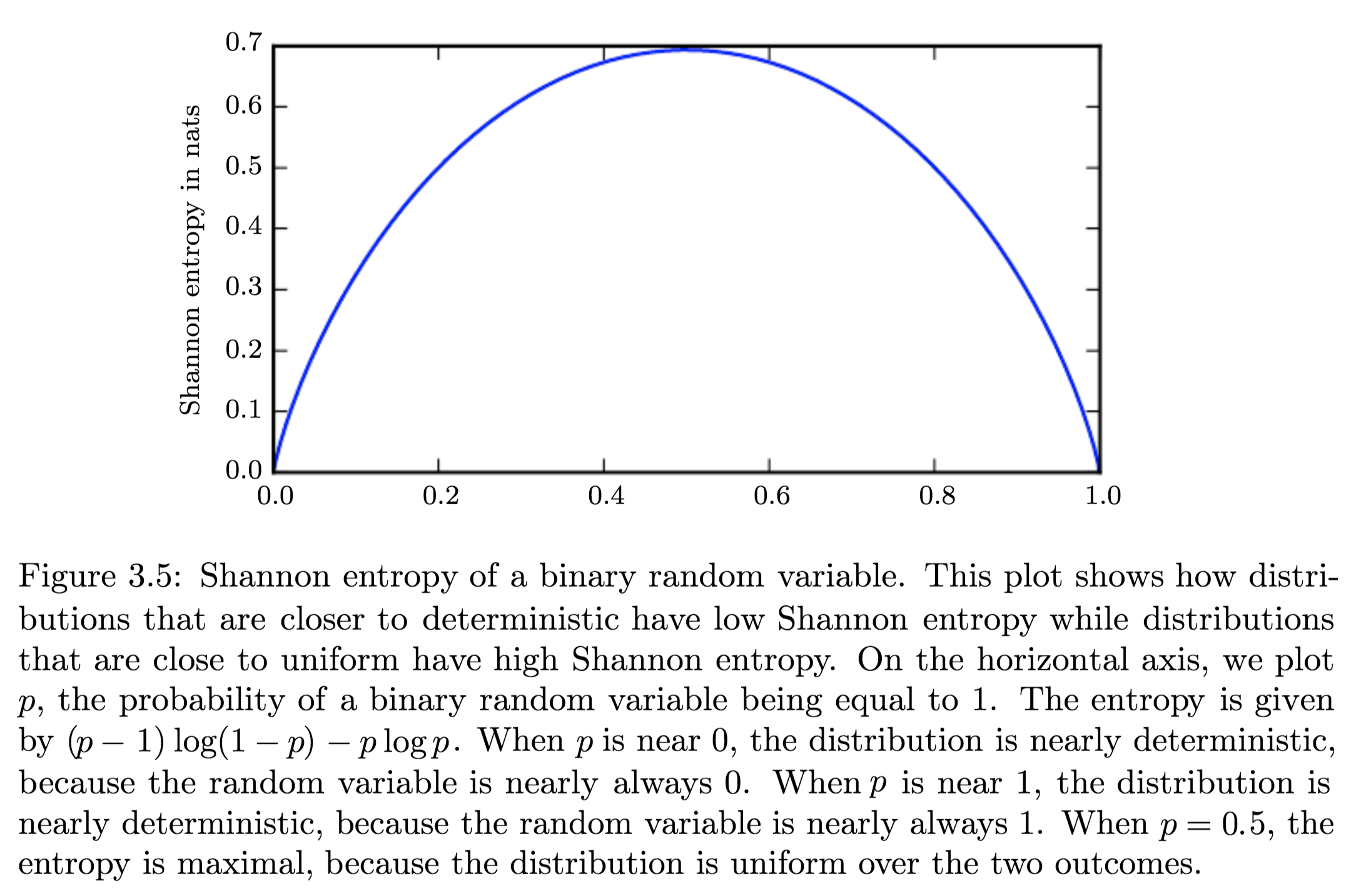
- Describe how Shannon Entropy relate to distributions with a graph:
- Define Differential Entropy:
Differential Entropy is Shannons entropy of a continuous random variable \(x\) - How does entropy characterize distributions?
Distributions that are nearly deterministic (where the outcome is nearly certain) have low entropy; distributions that are closer to uniform have high entropy. -
Define Relative Entropy - Give it’s formula:
The Kullback–Leibler divergence (Relative Entropy) is a measure of how one probability distribution diverges from a second, expected probability distribution.Mathematically:
$${\displaystyle D_{\text{KL}}(P\parallel Q)=\operatorname{E}_{x \sim P} \left[\log \dfrac{P(x)}{Q(x)}\right]=\operatorname{E}_{x \sim P} \left[\log P(x) - \log Q(x)\right]}$$
- Discrete:
$${\displaystyle D_{\text{KL}}(P\parallel Q)=\sum_{i}P(i)\log \left({\frac {P(i)}{Q(i)}}\right)}$$
- Continuous:
$${\displaystyle D_{\text{KL}}(P\parallel Q)=\int_{-\infty }^{\infty }p(x)\log \left({\frac {p(x)}{q(x)}}\right)\,dx,}$$
- Give an interpretation:
- Discrete variables:
It is the extra amount of information needed to send a message containing symbols drawn from probability distribution \(P\), when we use a code that was designed to minimize the length of messages drawn from probability distribution \(Q\).
- Discrete variables:
- List the properties:
- Non-Negativity:
\({\displaystyle D_{\mathrm {KL} }(P\|Q) \geq 0}\) - \({\displaystyle D_{\mathrm {KL} }(P\|Q) = 0 \iff}\) \(P\) and \(Q\) are:
- Discrete Variables:
the same distribution - Continuous Variables:
equal “almost everywhere”
- Discrete Variables:
- Additivity of Independent Distributions:
\({\displaystyle D_{\text{KL}}(P\parallel Q)=D_{\text{KL}}(P_{1}\parallel Q_{1})+D_{\text{KL}}(P_{2}\parallel Q_{2}).}\) - \({\displaystyle D_{\mathrm {KL} }(P\|Q) \neq D_{\mathrm {KL} }(Q\|P)}\)
This asymmetry means that there are important consequences to the choice of the ordering
- Convexity in the pair of PMFs \((p, q)\) (i.e. \({\displaystyle (p_{1},q_{1})}\) and \({\displaystyle (p_{2},q_{2})}\) are two pairs of PMFs):
\({\displaystyle D_{\text{KL}}(\lambda p_{1}+(1-\lambda )p_{2}\parallel \lambda q_{1}+(1-\lambda )q_{2})\leq \lambda D_{\text{KL}}(p_{1}\parallel q_{1})+(1-\lambda )D_{\text{KL}}(p_{2}\parallel q_{2}){\text{ for }}0\leq \lambda \leq 1.}\)
- Non-Negativity:
- Describe it as a distance:
Because the KL divergence is non-negative and measures the difference between two distributions, it is often conceptualized as measuring some sort of distance between these distributions.
However, it is not a true distance measure because it is not symmetric.KL-div is, however, a Quasi-Metric, since it satisfies all the properties of a distance-metric except symmetry
- List the applications of relative entropy:
Characterizing:- Relative (Shannon) entropy in information systems
- Randomness in continuous time-series
- Information gain when comparing statistical models of inference
- How does the direction of minimization affect the optimization:
Suppose we have a distribution \(p(x)\) and we wish to approximate it with another distribution \(q(x)\).
We have a choice of minimizing either:- \({\displaystyle D_{\text{KL}}(p\|q)} \implies q^\ast = \operatorname {arg\,min}_q {\displaystyle D_{\text{KL}}(p\|q)}\)
Produces an approximation that usually places high probability anywhere that the true distribution places high probability. - \({\displaystyle D_{\text{KL}}(q\|p)} \implies q^\ast \operatorname {arg\,min}_q {\displaystyle D_{\text{KL}}(q\|p)}\)
Produces an approximation that rarely places high probability anywhere that the true distribution places low probability.which are different due to the asymmetry of the KL-divergence
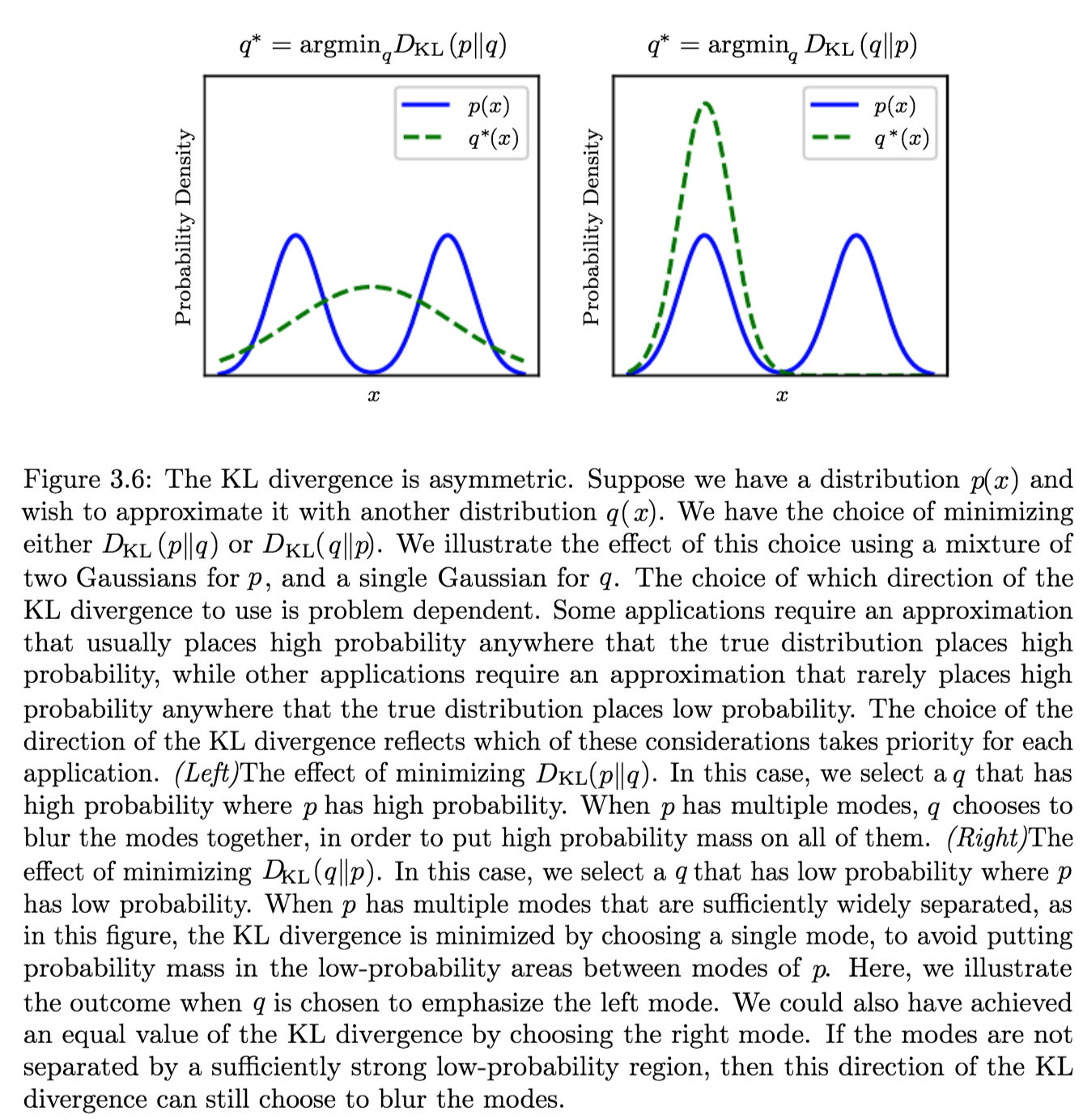
- \({\displaystyle D_{\text{KL}}(p\|q)} \implies q^\ast = \operatorname {arg\,min}_q {\displaystyle D_{\text{KL}}(p\|q)}\)
- Define Cross Entropy - Give it’s formula:
The Cross Entropy between two probability distributions \({\displaystyle p}\) and \({\displaystyle q}\) over the same underlying set of events measures the average number of bits needed to identify an event drawn from the set, if a coding scheme is used that is optimized for an “unnatural” probability distribution \({\displaystyle q}\), rather than the “true” distribution \({\displaystyle p}\).$$H(p,q) = \operatorname{E}_{p}[-\log q]= H(p) + D_{\mathrm{KL}}(p\|q) =-\sum_{x }p(x)\,\log q(x)$$
- What does it measure?
The average number of bits that need to be transmitted using a different probability distribution \(q\) (for encoding) than the “true” distribution \(p\), to convey the information in \(p\). - How does it relate to relative entropy?
It is similar to KL-Div but with an additional quantity - the entropy of \(p\). - When are they equivalent?
Minimizing the cross-entropy with respect to \(Q\) is equivalent to minimizing the KL divergence, because \(Q\) does not participate in the omitted term.
- What does it measure?
- Mutual Information:
- Definition:
The Mutual Information (MI) of two random variables is a measure of the mutual dependence between the two variables.
More specifically, it quantifies the “amount of information” (in bits) obtained about one random variable through observing the other random variable. - What does it measure?
It can be seen as a way of measuring the reduction in uncertainty (information content) of measuring a part of the system after observing the outcome of another parts of the system; given two R.Vs, knowing the value of one of the R.Vs in the system gives a corresponding reduction in (the uncertainty (information content) of) measuring the other one. - Intuitive Definitions:
- Measures the information that \(X\) and \(Y\) share:
It measures how much knowing one of these variables reduces uncertainty about the other.- \(X, Y\) Independent \(\implies I(X; Y) = 0\): their MI is zero
- \(X\) deterministic function of \(Y\) and vice versa \(\implies I(X; Y) = H(X) = H(Y)\) their MI is equal to entropy of each variable
- It’s a Measure of the inherent dependence expressed in the joint distribution of \(X\) and \(Y\) relative to the joint distribution of \(X\) and \(Y\) under the assumption of independence.
i.e. The price for encoding \({\displaystyle (X,Y)}\) as a pair of independent random variables, when in reality they are not.
- Measures the information that \(X\) and \(Y\) share:
- Properties:
- The KL-divergence shows that \(I(X; Y)\) is equal to zero precisely when the joint distribution conicides with the product of the marginals i.e. when \(X\) and \(Y\) are independent.
- The MI is non-negative: \(I(X; Y) \geq 0\)
- It is a measure of the price for encoding \({\displaystyle (X,Y)}\) as a pair of independent random variables, when in reality they are not.
- It is symmetric: \(I(X; Y) = I(Y; X)\)
- Related to conditional and joint entropies:
$${\displaystyle {\begin{aligned}\operatorname {I} (X;Y)&{}\equiv \mathrm {H} (X)-\mathrm {H} (X|Y)\\&{}\equiv \mathrm {H} (Y)-\mathrm {H} (Y|X)\\&{}\equiv \mathrm {H} (X)+\mathrm {H} (Y)-\mathrm {H} (X,Y)\\&{}\equiv \mathrm {H} (X,Y)-\mathrm {H} (X|Y)-\mathrm {H} (Y|X)\end{aligned}}}$$
where \(\mathrm{H}(X)\) and \(\mathrm{H}(Y)\) are the marginal entropies, \(\mathrm{H}(X | Y)\) and \(\mathrm{H}(Y | X)\) are the conditional entopries, and \(\mathrm{H}(X, Y)\) is the joint entropy of \(X\) and \(Y\).
- Note the analogy to the union, difference, and intersection of two sets:

- Note the analogy to the union, difference, and intersection of two sets:
- Related to KL-div of conditional distribution:
$$\mathrm{I}(X ; Y)=\mathbb{E}_{Y}\left[D_{\mathrm{KL}}\left(p_{X | Y} \| p_{X}\right)\right]$$
- Applications:
- In search engine technology, mutual information between phrases and contexts is used as a feature for k-means clustering to discover semantic clusters (concepts)
- Discriminative training procedures for hidden Markov models have been proposed based on the maximum mutual information (MMI) criterion.
- Mutual information has been used as a criterion for feature selection and feature transformations in machine learning. It can be used to characterize both the relevance and redundancy of variables, such as the minimum redundancy feature selection.
- Mutual information is used in determining the similarity of two different clusterings of a dataset. As such, it provides some advantages over the traditional Rand index.
- Mutual information of words is often used as a significance function for the computation of collocations in corpus linguistics.
- Detection of phase synchronization in time series analysis
- The mutual information is used to learn the structure of Bayesian networks/dynamic Bayesian networks, which is thought to explain the causal relationship between random variables
- Popular cost function in decision tree learning.
- In the infomax method for neural-net and other machine learning, including the infomax-based Independent component analysis algorithm
- As KL-Divergence:
Let \((X, Y)\) be a pair of random variables with values over the space \(\mathcal{X} \times \mathcal{Y}\) . If their joint distribution is \(P_{(X, Y)}\) and the marginal distributions are \(P_{X}\) and \(P_{Y},\) the mutual information is defined as:$$I(X ; Y)=D_{\mathrm{KL}}\left(P_{(X, Y)} \| P_{X} \otimes P_{Y}\right)$$
- In-terms of PMFs for discrete distributions:
The mutual information of two jointly discrete random variables \(X\) and \(Y\) is calculated as a double sum:$$\mathrm{I}(X ; Y)=\sum_{y \in \mathcal{Y}} \sum_{x \in \mathcal{X}} p_{(X, Y)}(x, y) \log \left(\frac{p_{(X, Y)}(x, y)}{p_{X}(x) p_{Y}(y)}\right)$$
where \({\displaystyle p_{(X,Y)}}\) is the joint probability mass function of \({\displaystyle X}\) X and \({\displaystyle Y}\), and \({\displaystyle p_{X}}\) and \({\displaystyle p_{Y}}\) are the marginal probability mass functions of \({\displaystyle X}\) and \({\displaystyle Y}\) respectively.
- In terms of PDFs for continuous distributions:
In the case of jointly continuous random variables, the double sum is replaced by a double integral:$$\mathrm{I}(X ; Y)=\int_{\mathcal{Y}} \int_{\mathcal{X}} p_{(X, Y)}(x, y) \log \left(\frac{p_{(X, Y)}(x, y)}{p_{X}(x) p_{Y}(y)}\right) d x d y$$
where \(p_{(X, Y)}\) is now the joint probability density function of \(X\) and \(Y\) and \(p_{X}\) and \(p_{Y}\) are the marginal probability density functions of \(X\) and \(Y\) respectively.
- Relation to PMI:
The mutual information (MI) of the random variables \(X\) and \(Y\) is the expected value of the PMI (over all possible outcomes).
- Definition:
- Pointwise Mutual Information (PMI):
- Definition:
The PMI of a pair of outcomes \(x\) and \(y\) belonging to discrete random variables \(X\) and \(Y\) quantifies the discrepancy between the probability of their coincidence given their joint distribution and their individual distributions, assuming independence. Mathematically:$$\operatorname{pmi}(x ; y) \equiv \log \frac{p(x, y)}{p(x) p(y)}=\log \frac{p(x | y)}{p(x)}=\log \frac{p(y | x)}{p(y)}$$
- Relation to MI:
In contrast to mutual information (MI) which builds upon PMI, it refers to single events, whereas MI refers to the average of all possible events.
The mutual information (MI) of the random variables \(X\) and \(Y\) is the expected value of the PMI (over all possible outcomes).
- Definition:
Recommendation Systems
- Describe the different algorithms for recommendation systems:
Ensemble Learning
- What are the two paradigms of ensemble methods?
- Parallel
- Sequential
- Random Forest VS GBM?
The fundamental difference is, random forest uses bagging technique to make predictions. GBM uses boosting techniques to make predictions.
Data Processing and Analysis
- What are 3 data preprocessing techniques to handle outliers?
- Winsorizing/Winsorization (cap at threshold).
- Transform to reduce skew (using Box-Cox or similar).
- Remove outliers if you’re certain they are anomalies or measurement errors.
- Describe the strategies to dimensionality reduction?
- Feature Selection
- Feature Projection/Extraction
- What are 3 ways of reducing dimensionality?
- Removing Collinear Features
- Performing PCA, ICA, etc.
- Feature Engineering
- AutoEncoder
- Non-negative matrix factorization (NMF)
- LDA
- MSD
- List methods for Feature Selection
- Variance Threshold: normalize first (variance depends on scale)
- Correlation Threshold: remove the one with larger mean absolute correlation with other features.
- Genetic Algorithms
- Stepwise Search: bad performance, regularization much better, it’s a greedy algorithm (can’t account for future effects of each change)
- LASSO, Elastic-Net
- List methods for Feature Extraction
- PCA, ICA, CCA
- AutoEncoders
- LDA: LDA is a supervised linear transformation technique since the dependent variable (or the class label) is considered in the model. It Extracts the k new independent variables that maximize the separation between the classes of the dependent variable.
- Linear discriminant analysis is used to find a linear combination of features that characterizes or separates two or more classes (or levels) of a categorical variable.
- Unlike PCA, LDA extracts the k new independent variables that maximize the separation between the classes of the dependent variable. LDA is a supervised linear transformation technique since the dependent variable (or the class label) is considered in the model.
- Latent Semantic Analysis
- Isomap
- How to detect correlation of “categorical variables”?
- Chi-Squared test: it is a statistical test applied to the groups of categorical features to evaluate the likelihood of correlation or association between them using their frequency distribution.
- Feature Importance
- Use linear regression and select variables based on \(p\) values
- Use Random Forest, Xgboost and plot variable importance chart
- Lasso
- Measure information gain for the available set of features and select top \(n\) features accordingly.
- Use Forward Selection, Backward Selection, Stepwise Selection
- Remove the correlated variables prior to selecting important variables
- In linear models, feature importance can be calculated by the scale of the coefficients
- In tree-based methods (such as random forest), important features are likely to appear closer to the root of the tree. We can get a feature’s importance for random forest by computing the averaging depth at which it appears across all trees in the forest
- Capturing the correlation between continuous and categorical variable? If yes, how?
Yes, we can use ANCOVA (analysis of covariance) technique to capture association between continuous and categorical variables.
ANCOVA Explained - What cross validation technique would you use on time series data set?
Forward chaining strategy with k folds. - How to deal with missing features? (Imputation?)
- Assign a unique category to missing values, who knows the missing values might decipher some trend.
- Remove them blatantly
- we can sensibly check their distribution with the target variable, and if found any pattern we’ll keep those missing values and assign them a new category while removing others.
- Do you suggest that treating a categorical variable as continuous variable would result in a better predictive model?
For better predictions, categorical variable can be considered as a continuous variable only when the variable is ordinal in nature. - What are collinearity and multicollinearity?
- Collinearity occurs when two predictor variables (e.g., \(x_1\) and \(x_2\)) in a multiple regression have some correlation.
- Multicollinearity occurs when more than two predictor variables (e.g., \(x_1, x_2, \text{ and } x_3\)) are inter-correlated.
- What is data normalization and why do we need it?
ML/Statistical Models
- What are parametric models?
Parametric models are those with a finite number of parameters. To predict new data, you only need to know the parameters of the model. Examples include linear regression, logistic regression, and linear SVMs. - What is a classifier?
A function that maps…
K-NN
PCA
- What is PCA?
It is a statistical procedure that uses an orthogonal transformation to convert a set of observations of possibly correlated variables into a set of values of linearly uncorrelated variables called principal components. - What is the Goal of PCA?
Given points \(\mathbf{x}_ i \in \mathbf{R}^d\), find k-directions that capture most of the variation. - List the applications of PCA:
- Find a small basis for representing variations in complex things.
e.g. faces, genes.
- Reducing the number of dimensions makes some computations cheaper.
- Remove irrelevant dimensions to reduce over-fitting in learning algorithms.
Like “subset selection” but the features are not axis aligned.
They are linear combinations of input features. - Represent the data with fewer parameters (dimensions)
- Find a small basis for representing variations in complex things.
- Give formulas for the following:
- Assumptions on \(X\):
The analysis above is valid only for (1) \(X\) w/ samples in rows and variables in columns (2) \(X\) is centered (mean=0) - SVD of \(X\):
\(X = USV^{T}\) - Principal Directions/Axes:
\(V\) - Principal Components (scores):
\(US\) - The \(j\)-th principal component:
\(Xv_j = Us_j\)
- Assumptions on \(X\):
- Define the transformation, mathematically:
Mathematically, the transformation is defined by a set of \(p\)-dimensional vectors of weights or coefficients \({\displaystyle \mathbf {v}_ {(k)}=(v_{1},\dots ,v_{p})_ {(k)}}\) that map each row vector \({\displaystyle \mathbf {x}_ {(i)}}\) of \(X\) to a new vector of principal component scores \({\displaystyle \mathbf {t} _{(i)}=(t_{1},\dots ,t_{l})_ {(i)}}\), given by:$${\displaystyle {t_{k}}_{(i)}=\mathbf {x}_ {(i)}\cdot \mathbf {v}_ {(k)}\qquad \mathrm {for} \qquad i=1,\dots ,n\qquad k=1,\dots ,l}$$
in such a way that the individual variables \({\displaystyle t_{1},\dots ,t_{l}}\) of \(t\) considered over the data set successively inherit the maximum possible variance from \(X\), with each coefficient vector \(v\) constrained to be a unit vector (where \(l\) is usually selected to be less than \({\displaystyle p}\) to reduce dimensionality).
- What does PCA produce/result in?
- Finds a lower dimensional subspace spanned by what?:
Finds a lower dimensional subspace spanned by PCs. - Finds a lower dimensional subspace that minimizes what?:
Finds a lower dimensional subspace (PCs) that Minimizes the RSS of projection errors. - What does each PC have (properties)?
Produces a vector (1st PC) with the highest possible variance, each succeeding component in turn has the highest variance possible under the constraint that it is orthogonal to the preceding components. - What does the procedure find in terms of a “basis”?
Results in an uncorrelated orthogonal basis set. - What does the procedure find in terms of axes? (where do they point?):
PCA constructs new axes that point to the directions of maximal variance (in the original variable space)
- Finds a lower dimensional subspace spanned by what?:
- Describe the PCA algorithm:
- Data Preprocessing:
- Training set: \(x^{(1)}, x^{(2)}, \ldots, x^{(m)}\)
- Preprocessing (feature scaling + mean normalization):
- mean normalization:
\(\mu_{j}=\frac{1}{m} \sum_{i=1}^{m} x_{j}^{(i)}\)
Replace each \(x_{j}^{(i)}\) with \(x_j^{(i)} - \mu_j\) - feature scaling:
If different features on different, scale features to have comparable range
\(s_j = S.D(X_j)\) (the standard deviation of feature \(j\))
Replace each \(x_{j}^{(i)}\) with \(\dfrac{x_j^{(i)} - \mu_j}{s_j}\)
- mean normalization:
- Computing the Principal Components:
- Compute the SVD of the matrix \(X = U S V^T\)
- Compute the Principal Components:
$$T = US = XV$$
Note: The \(j\)-th principal component is: \(Xv_j\)
- Choose the top \(k\) components singular values in \(S = S_k\)
- Compute the Truncated Principal Components:
$$T_k = US_k$$
- Computing the Low-rank Approximation Matrix \(X_k\):
- Compute the reconstruction matrix:
$$X_k = T_kV^T = US_kV^T$$
- Compute the reconstruction matrix:
- What Data Processing needs to be done?
- Preprocessing (feature scaling + mean normalization):
- mean normalization:
\(\mu_{j}=\frac{1}{m} \sum_{i=1}^{m} x_{j}^{(i)}\)
Replace each \(x_{j}^{(i)}\) with \(x_j^{(i)} - \mu_j\) - feature scaling:
If different features on different, scale features to have comparable range
\(s_j = S.D(X_j)\) (the standard deviation of feature \(j\))
Replace each \(x_{j}^{(i)}\) with \(\dfrac{x_j^{(i)} - \mu_j}{s_j}\)
- mean normalization:
- Preprocessing (feature scaling + mean normalization):
- How to compute the Principal Components?
- Compute the SVD of the matrix \(X = U S V^T\)
- Compute the Principal Components:
$$T = US = XV$$
- How do you compute the Low-Rank Approximation Matrix \(X_k\)?
- Choose the top \(k\) components singular values in \(S = S_k\)
- Compute the Truncated Principal Components:
$$T_k = US_k$$
- Compute the reconstruction matrix:
$$X_k = T_kV^T = US_kV^T$$
- Data Preprocessing:
- Describe the Optimality of PCA:
Optimal for Finding a lower dimensional subspace (PCs) that Minimizes the RSS of projection errors. - List limitations of PCA:
- PCA is highly sensitive to the (relative) scaling of the data; no consensus on best scaling.
- Intuition:
- PCA can be thought of as fitting a \(p\)-dimensional ellipsoid to the data, where each axis of the ellipsoid represents a principal component. If some axis of the ellipsoid is small, then the variance along that axis is also small, and by omitting that axis and its corresponding principal component from our representation of the dataset, we lose only a commensurately small amount of information.
- Its operation can be thought of as revealing the internal structure of the data in a way that best explains the variance in the data.
- What property of the internal structure of the data does PCA reveal/explain?
The variance in the data. - What object does it fit to the data?:
- PCA can be thought of as fitting a \(p\)-dimensional ellipsoid to the data, where each axis of the ellipsoid represents a principal component.
- Should you remove correlated features b4 PCA?
Yes. Discarding correlated variables have a substantial effect on PCA because, in presence of correlated variables, the variance explained by a particular component gets inflated. Discussion - How can we measure the “Total Variance” of the data?
1.*The Total Variance** of the data can be expressed as the sum of all the eigenvalues:$$\mathbf{Tr} \Sigma = \mathbf{Tr} (U \Lambda U^T) = \mathbf{Tr} (U^T U \Lambda) = \mathbf{Tr} \Lambda = \lambda_1 + \ldots + \lambda_n.$$
- How can we measure the “Total Variance” of the projected data?
1.*The Total Variance** of the Projected data is:$$\mathbf{Tr} (P \Sigma P^T ) = \lambda_1 + \lambda_2 + \cdots + \lambda_k. $$
- How can we measure the “Error in the Projection”?
1.*The Error in the Projection** could be measured with respect to variance.- We define the ratio of variance “explained” by the projected data (equivalently, the ratio of information “retained”) as:
$$\dfrac{\lambda_1 + \ldots + \lambda_k}{\lambda_1 + \ldots + \lambda_n}. $$
- What does it mean when this ratio is high?
If the ratio is high, we can say that much of the variation in the data can be observed on the projected plane.
- How does PCA relate to CCA?
- CCA defines coordinate systems that optimally describe the cross-covariance between two datasets while
- PCA defines a new orthogonal coordinate system that optimally describes variance in a single dataset.
- How does PCA relate to ICA?
Independent component analysis (ICA) is directed to similar problems as principal component analysis, but finds additively separable components rather than successive approximations.
The Centroid Method
-
Define “The Centroid”:
In mathematics and physics, the centroid or geometric center of a plane figure is the arithmetic mean (“average”) position of all the points in the shape.The definition extends to any object in n-dimensional space: its centroid is the mean position of all the points in all of the coordinate directions.
-
Describe the Procedure:
Compute the mean (\(\mu_c\)) of all the vectors in class \(C\) and the mean (\(\mu_x\)) of all the vectors not in \(C\) - What is the Decision Function:
$$f(x) = (\mu_c - \mu_x) \cdot \vec{x} - (\mu_c - \mu_x) \cdot \dfrac{\mu_c + \mu_x}{2}$$
- Describe the Decision Boundary:
The decision boundary is a Hyperplane that bisects the line segment with endpoints \(<\mu_c, \mu_x>\)
K-Means
- What is K-Means?
It is a clustering algorithm. It aims to partition \(n\) observations into \(k\) clusters in which each observation belongs to the cluster with the nearest mean. It results in a partitioning of the data space into Voronoi Cells. - What is the idea behind K-Means?
- Minimize the aggregate intra-cluster distance
- Equivalent to minimizing the variance
- Thus, it finds \(k-\)clusters with minimum aggregate variance
- What does K-Mean find?
It finds \(k-\)clusters with minimum aggregate variance. - Formal Description of the Model:
Given a set of observations \(\left(\mathbf{x}_{1}, \mathbf{x} _{2}, \ldots, \mathbf{x}_{n}\right)\), \(\mathbf{x}_ i \in \mathbb{R}^d\), the algorithm aims to partition the \(n\) observations into \(k\) sets \(\mathbf{S}=\left\{S_{1}, S_{2}, \ldots, S_{k}\right\}\) so as to minimize the intra-cluster Sum-of-Squares (i.e. variance).- What is the Objective?
$$\underset{\mathbf{S}}{\arg \min } \sum_{i=1}^{k} \sum_{\mathbf{x} \in S_{i}}\left\|\mathbf{x}-\boldsymbol{\mu}_{i}\right\|^{2}=\underset{\mathbf{S}}{\arg \min } \sum_{i=1}^{k}\left|S_{i}\right| \operatorname{Var} S_{i}$$
where \(\boldsymbol{\mu}_i\) is the mean of points in \(S_i\).
- What is the Objective?
- Description of the Algorithm:
- Choose two random points, call them “Centroids”
- Assign the closest \(N/2\) points (Euclidean-wise) to each of the Centroids
- Compute the mean of each “group”/class of points
- Re-Assign the centroids to the newly computed Means ↑
- REPEAT!
- What is the Optimization method used? What class does it belong to?
Coordinate descent. Expectation-Maximization.
- How does the optimization method relate to EM?
The “assignment” step is referred to as the “expectation step”, while the “update step” is a maximization step, making this algorithm a variant of the generalized expectation-maximization algorithm.
- How does the optimization method relate to EM?
- What is the Complexity of the algorithm?
The original formulation of the problem is NP-Hard; however, EM algorithms (specifically, Coordinate-Descent) can be used as efficient heuristic algorithms that converge quickly to good local minima. - Describe the convergence and prove it:
Guaranteed to converge after a finite number of iterations to a local minimum.-
Proof:
The Algorithm Minimizes a monotonically decreasing, Non-Negative Energy function on a finite Domain:
By Monotone Convergence Theorem the objective Value Converges.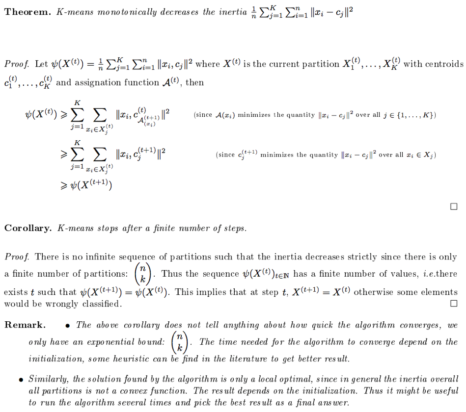
-
- Describe the Optimality of the Algorithm:
- Locally optimal:
due to convergence property - Non-Globally optimal:
- The objective function is non-convex
- Moreover, coordinate Descent doesn’t converge to global minimum on non-convex functions.
- Locally optimal:
- Derive the estimated parameters of the algorithm:
- Objective Function:
$$J(S, \mu)= \sum_{i=1}^{k} \sum_{\mathbf{x} \in S_{i}} \| \mathbf{x} -\mu_i \|^{2}$$
- Optimization Objective:
$$\min _{\mu} \min _{S} \sum_{i=1}^{k} \sum_{\mathbf{x} \in S_{i}}\left\|\mathbf{x} -\mu_{i}\right\|^{2}$$
- Derivation:
- Fix \(S = \hat{S}\), optimize \(\mu\):
$$\begin{aligned} & \min _{\mu} \sum_{i=1}^{k} \sum_{\mathbf{x} \in \hat{S}_{i}}\left\|\mu_{i}-x_{j}\right\|^{2}\\ =& \sum_{i=1}^{k} \min _{\mu_i} \sum_{\mathbf{x} \in \hat{S}_{i}}\left\|\mathbf{x} - \mu_{i}\right\|^{2} \end{aligned}$$
- MLE:
$$\min _{\mu_i} \sum_{\mathbf{x} \in \hat{S}_{i}}\left\|\mathbf{x} - \mu_{i}\right\|^{2}$$
\(\implies\)
$${\displaystyle \hat{\mu_i} = \dfrac{\sum_{\mathbf{x} \in \hat{S}_ {i}} \mathbf{x}}{\vert\hat{S}_ i\vert}}$$
- MLE:
- Fix \(\mu_i = \hat{\mu_i}, \forall i\), optimize \(S\):
$$\arg \min _{S} \sum_{i=1}^{k} \sum_{\mathbf{x} \in S_{i}}\left\|\mathbf{x} - \hat{\mu_{i}}\right\|^{2}$$
\(\implies\)
$$S_{i}^{(t)}=\left\{x_{p} :\left\|x_{p}-m_{i}^{(t)}\right\|^{2} \leq\left\|x_{p}-m_{j}^{(t)}\right\|^{2} \forall j, 1 \leq j \leq k\right\}$$
- MLE:
- MLE:
- Objective Function:
- When does K-Means fail to give good results?
K-means clustering algorithm fails to give good results when:- the data contains outliers
- the density spread of data points across the data space is different
- and the data points follow nonconvex shapes.
Naive Bayes
- Define:
- Naive Bayes:
It is a simple technique used for constructing classifiers. - Naive Bayes Classifiers:
A family of simple probabilistic classifiers based on applying bayes theorem with strong (naive) independence assumptions between the features. - Bayes Theorem:
\(p(x\vert y) = \dfrac{p(y\vert x) p(x)}{p(y)}\)
- Naive Bayes:
- List the assumptions of Naive Bayes:
- Conditional Independence: the features are conditionally independent from each other given a class \(C_k\)
- Bag-of-words: The relative importance (positions) of the features do not matter
- List some properties of Naive Bayes:
- Not a Bayesian method
- It’s a Bayes Classifier: minimizes the probability of misclassification
- Is it a Bayesian Method or Frequentest Method?
Not a Bayesian method - Is it a Bayes Classifier? What does that mean?:
It’s a Bayes Classifier: minimizes the probability of misclassification
- Define the Probabilistic Model for the method:
Naive Bayes is a conditional probability model:
given a problem instance to be classified represented by a vector \(\boldsymbol{x} = (x_1, \cdots, x_n)\) of \(n\) features/words (independent variables), it assigns to this instance probabilities:$$P(C_k\vert \boldsymbol{x}) = p(C_k\vert x_1, \cdots, x_n)$$
for each of the \(k\) classes.
Using Bayes theorem to decompose the conditional probability:
$$p(C_k\vert \boldsymbol{x}) = \dfrac{p(\boldsymbol{x}\vert C_k) p(C_k)}{p(\boldsymbol{x})}$$
Notice that the numerator is equivalent to the joint probability distribution:
$$p\left(C_{k}\right) p\left(\mathbf{x} | C_{k}\right) = p\left(C_{k}, x_{1}, \ldots, x_{n}\right)$$
Using the Chain-Rule for repeated application of the conditional probability, the joint probability model can be rewritten as:
$$p(C_{k},x_{1},\dots ,x_{n})\, = p(x_{1}\mid x_{2},\dots ,x_{n},C_{k})p(x_{2}\mid x_{3},\dots ,x_{n},C_{k})\dots p(x_{n-1}\mid x_{n},C_{k})p(x_{n}\mid C_{k})p(C_{k})$$
Using the Naive Conditional Independence assumptions:
$$p\left(x_{i} | x_{i+1}, \ldots, x_{n}, C_{k}\right)=p\left(x_{i} | C_{k}\right)$$
Thus, we can write the joint model as:
$${\displaystyle {\begin{aligned}p(C_{k}\mid x_{1},\dots ,x_{n})&\varpropto p(C_{k},x_{1},\dots ,x_{n})\\&=p(C_{k})\ p(x_{1}\mid C_{k})\ p(x_{2}\mid C_{k})\ p(x_{3}\mid C_{k})\ \cdots \\&=p(C_{k})\prod _{i=1}^{n}p(x_{i}\mid C_{k})\,,\end{aligned}}}$$
Finally, the conditional distribution over the class variable \(C\) is:
$${\displaystyle p(C_{k}\mid x_{1},\dots ,x_{n})={\frac {1}{Z}}p(C_{k})\prod _{i=1}^{n}p(x_{i}\mid C_{k})}$$
where, \({\displaystyle Z=p(\mathbf {x} )=\sum _{k}p(C_{k})\ p(\mathbf {x} \mid C_{k})}\) is a constant scaling factor, a dependent only on the, known, feature variables \(x_i\)s.
- What kind of model is it?
Conditional Probability Model. - What is a conditional probability model?
A model that assigns probabilities to an input \(\boldsymbol{x}\) conditioned on being a member of each class in a set of \(k\) classes \(C_1, \cdots, C_k\). - Decompose the conditional probability w/ Bayes Theorem:
$$p(C_k\vert \boldsymbol{x}) \dfrac{p(\boldsymbol{x}\vert C_k) p(C_k)}{p(\boldsymbol{x})}= $$
- How does the new expression incorporate the joint probability model?
We notice that the numerator is equivalent to the joint probability distribution:$$p\left(C_{k}\right) p\left(\mathbf{x} | C_{k}\right) = p\left(C_{k}, x_{1}, \ldots, x_{n}\right)$$
- Use the chain rule to re-write the joint probability model:
$$p(C_{k},x_{1},\dots ,x_{n})\, = p(x_{1}\mid x_{2},\dots ,x_{n},C_{k})p(x_{2}\mid x_{3},\dots ,x_{n},C_{k})\dots p(x_{n-1}\mid x_{n},C_{k})p(x_{n}\mid C_{k})p(C_{k})$$
- Use the Naive Conditional Independence assumption to rewrite the joint model:
$${\displaystyle {\begin{aligned}p(C_{k}\mid x_{1},\dots ,x_{n})&\varpropto p(C_{k},x_{1},\dots ,x_{n})\\&=p(C_{k})\ p(x_{1}\mid C_{k})\ p(x_{2}\mid C_{k})\ p(x_{3}\mid C_{k})\ \cdots \\&=p(C_{k})\prod _{i=1}^{n}p(x_{i}\mid C_{k})\,,\end{aligned}}}$$
- What is the conditional distribution over the class variable \(C_k\):
$${\displaystyle p(C_{k}\mid x_{1},\dots ,x_{n})={\frac {1}{Z}}p(C_{k})\prod _{i=1}^{n}p(x_{i}\mid C_{k})}$$
where, \({\displaystyle Z=p(\mathbf {x} )=\sum _{k}p(C_{k})\ p(\mathbf {x} \mid C_{k})}\) is a constant scaling factor, a dependent only on the, known, feature variables \(x_i\)s.
- What kind of model is it?
-
Construct the classifier. What are its components? Formally define it.
The classifier is made of (1) the conditional probability model (above) \(\:\) and (2) A decision rule.The decision rule used is the MAP hypothesis: i.e. pick the hypothesis that is most probable (maximize the MAP estimate=posterior*prior).
The classifier is the function that assigns a class label \(\hat{y} = C_k\) for some \(k\) as follows:
$$\hat{y}=\underset{k \in\{1, \ldots, K\}}{\operatorname{argmax}} p\left(C_{k}\right) \prod_{i=1}^{n} p\left(x_{i} | C_{k}\right)$$
- What’s the decision rule used?
we commonly use the Maximum A Posteriori (MAP) hypothesis, as the decision rule; i.e. pick the hypothesis that is most probable. - List the difference between the Naive Bayes Estimate and the MAP Estimate:
- MAP Estimate:
$${\displaystyle {\hat {y}_{\text{MAP}}}={\underset {k\in \{1,\dots ,K\}}{\operatorname {argmax} }}\ p(C_{k})\ p(\mathbf {x} \mid C_{k})}$$
- Naive Bayes Estimate:
$${\displaystyle {\hat {y}_{\text{NB}}}={\underset {k\in \{1,\dots ,K\}}{\operatorname {argmax} }}\ p(C_{k})\displaystyle \prod _{i=1}^{n}p(x_{i}\mid C_{k})}$$
- MAP Estimate:
- What’s the decision rule used?
- What are the parameters to be estimated for the classifier?:
- The posterior probability of each feature/word given a class
- The prior probability of each class
- What method do we use to estimate the parameters?:
Maximum Likelihood Estimation (MLE). - What are the estimates for each of the following parameters?:
- The prior probability of each class:
\(\hat{P}(C_k) = \dfrac{\text{doc-count}(C=C_k)}{N_\text{doc}}\), - The conditional probability of each feature (word) given a class:
\(\hat{P}(x_i | C_i) = \dfrac{\text{count}(x_i,C_j)}{\sum_{x \in V} \text{count}(x, C_j)}\)
- The prior probability of each class:
CNNs
-
What is a CNN?
A convolutional neural network (CNN, or ConvNet) is a class of deep, feed-forward artificial neural networks that has successfully been applied to analyzing visual imagery.Convolutional networks are simply neural networks that use convolution in place of general matrix multiplication in at least one of their layers.
- What kind of data does it work on? What is the mathematical property?
In general, it works on data that have grid-like topology.
- What kind of data does it work on? What is the mathematical property?
- What are the layers of a CNN?
$$\text{Input} \longrightarrow \left[\text{Conv} \rightarrow \text{ReLU} \rightarrow \text{Pooling} \rightarrow \text{Norm}\right] \times N \longrightarrow \text{FC}$$
- What are the four important ideas and their benefits that the convolution affords CNNs:
-
Sparse Interactions/Connectivity/Weights:
Unlike FNNs, where every input unit is connected to every output unit, CNNs have sparse interactions. This is accomplished by making the kernel smaller than the input.Benefits:
- This means that we need to store fewer parameters, which both,
- Reduces the memory requirements of the model and
- Improves its statistical efficiency
- Also, Computing the output requires fewer operations
- In deep CNNs, the units in the deeper layers interact indirectly with large subsets of the input which allows modelling of complex interactions through sparse connections.
- This means that we need to store fewer parameters, which both,
-
Parameter Sharing:
refers to using the same parameter for more than one function in a model.Benefits:
- This means that rather than learning a separate set of parameters for every location, we learn only one set of parameters.
- This does not affect the runtime of forward propagation—it is still \(\mathcal{O}(k \times n)\)
- But it does further reduce the storage requirements of the model to \(k\) parameters (\(k\) is usually several orders of magnitude smaller than \(m\))
- This means that rather than learning a separate set of parameters for every location, we learn only one set of parameters.
-
Equivariant Representations:
For convolutions, the particular form of parameter sharing causes the layer to have a property called equivariance to translation.Thus, if we move the object in the input, its representation will move the same amount in the output.
Benefits:
- It is most useful when we know that some function of a small number of neighboring pixels is useful when applied to multiple input locations (e.g. edge detection)
- Shifting the position of an object in the input doesn’t confuse the NN
- Robustness against translated inputs/images
-
Accepts inputs of variable sizes
-
- What is the inspirational model for CNNs:
Convolutional networks were inspired by biological processes in which the connectivity pattern between neurons is inspired by the organization of the animal visual cortex.
Individual cortical neurons respond to stimuli only in a restricted region of the visual field known as the receptive field. The receptive fields of different neurons partially overlap such that they cover the entire visual field. - Describe the connectivity pattern of the neurons in a layer of a CNN:
The neurons in a layer will only be connected to a small region of the layer before it, instead of all of the neurons in a fully-connected manner. - Describe the process of a ConvNet:
ConvNets transform the original image layer by layer from the original pixel values to the final class scores. - Convolution Operation:
-
Define:
- Formula (continuous):
- Formula (discrete):
- Define the following:
- Feature Map:
- Does the operation commute?
-
- Cross Correlation:
- Define:
- Formulae:
- What are the differences/similarities between convolution and cross-correlation:
- Write down the Convolution operation and the cross-correlation over two axes and:
- Convolution:
- Convolution (commutative):
- Cross-Correlation:
- The Convolutional Layer:
- What are the parameters and how do we choose them?
- Describe what happens in the forward pass:
- What is the output of the forward pass:
- How is the output configured?
- Spatial Arrangements:
- List the Three Hyperparameters that control the output volume:
- How to compute the spatial size of the output volume?
- How can you ensure that the input & output volume are the same?
- In the output volume, how do you compute the \(d\)-th depth slice:
- Calculate the number of parameters for the following config:
Given:
1. Input Volume: \(64\times64\times3\)
1. Filters: \(15 7\times7\)
1. Stride: \(2\)
1. Pad: \(3\) - Definitions:
- Receptive Field:
- Suppose the input volume has size \([ 32 × 32 × 3 ]\) and the receptive field (or the filter size) is \(5 × 5\) , then each neuron in the Conv Layer will have weights to a __Blank__ region in the input volume, for a total of __Blank__ weights:
- How can we achieve the greatest reduction in the spatial dims of the network (for classification):
- Pooling Layer:
- Define:
- List key ideas/properties and benefits:
- List the different types of Pooling:
Answer - List variations of pooling and their definitions:
- What is “Learned Pooling”:
- What is “Dynamical Pooling”:
- List the hyperparams of Pooling Layer:
- How to calculate the size of the output volume:
- How many parameters does the pooling layer have:
- What are other ways to perform downsampling:
- Weight Priors:
- Define “Prior Prob Distribution on the parameters”:
- Define “Weight Prior” and its types/classes:
- Weak Prior:
- Strong Prior:
- Infinitely Strong Prior:
- Describe the Conv Layer as a FC Layer using priors:
- What are the key insights of using this view:
- When is the prior imposed by convolution INAPPROPRIATE:
- What happens when the priors imposed by convolution and pooling are not suitable for the task?
- What kind of other models should Convolutional models be compared to? Why?:
- When do multi-channel convolutions commute?
Answer - Why do we use several different kernels in a given conv-layer?
- Strided Convolutions
- Define:
- What are they used for?
- What are they equivalent to?
- Formula:
- Zero-Padding:
- Definition/Usage:
- List the types of padding:
- Locally Connected Layers/Unshared Convolutions:
- Bias Parameter:
- How many bias terms are used per output channel in the tradional convolution:
- Dilated Convolutions
- Define:
- What are they used for?
- Stacked Convolutions
- Define:
- What are they used for?
Theory
RNNs
- What is an RNN?
- Definition:
Recurrent Neural Networks (RNNs) are a family of neural networks for processing sequential data. - What machine-type is the standard RNN? What is its function?
The standard RNN is a nonlinear dynamical system that maps sequences to sequences. - Describe the connections in an RNN? Why does it matter?
In an RNN, the connections between units form a directed cycle, allowing it to exhibit dynamic temporal behavior.
- Definition:
- What is the big idea behind RNNs?
RNNs share parameters across different time-steps of the sequence, which allows it to generalize well to examples of different sequence length.
Such sharing is particularly important when a specific piece of information can occur at multiple positions within the sequence. - Dynamical Systems:
- Standard Form (equation and graph):
$$\boldsymbol{s}^{(t)}=f\left(\boldsymbol{s}^{(t-1)} ; \boldsymbol{\theta}\right) \tag{10.1}$$
where \(\boldsymbol{s}^{(t)}\) is called the state of the system.
- Standard Form with an external signal:
$$\boldsymbol{s}^{(t)}=f\left(\boldsymbol{s}^{(t-1)}, \boldsymbol{x}^{(t)} ; \boldsymbol{\theta}\right) \tag{10.4}$$
where \(\boldsymbol{x}^{(t)}\) is an external signal, and the state now contains information about the whole past sequence.
- RNN as a Dynamical System (eq+graph):
$$\boldsymbol{h}^{(t)}=f\left(\boldsymbol{h}^{(t-1)}, \boldsymbol{x}^{(t)} ; \boldsymbol{\theta}\right) \tag{10.5}$$
where the variable \(\mathbf{h}\) represents the state.
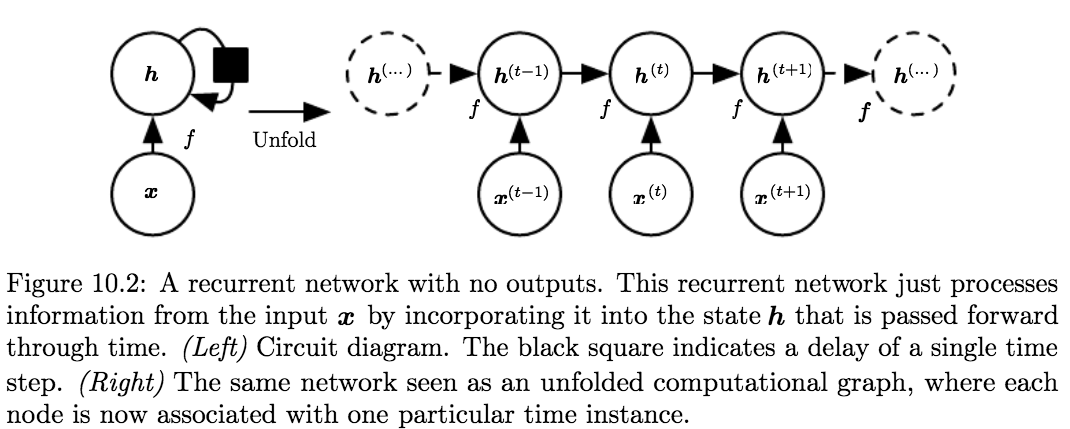
- What type of functions can be considered RNNs? (what property)
Basically, any function containing recurrence can be considered an RNN.
- Standard Form (equation and graph):
- Unfolding Computational Graphs
- Definition:
Unfolding maps the left to the right in the figure below (from figure 10.2) (both are computational graphs of a RNN without output \(\mathbf{o}\)):
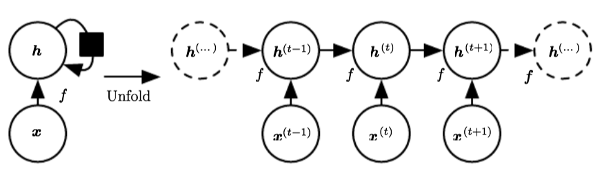
where the black square indicates that an interaction takes place with a delay of \(1\) time step, from the state at time \(t\) to the state at time \(t + 1\). - List the Advantages introduced by unfolding and the benefits:
- Regardless of the sequence length, the learned model always has the same input size.
Because it is specified in terms of transition from one state to another state, rather than specified in terms of a variable-length history of states. - It is possible to use the same transition function \(f\) with the same parameters at every time step.
Thus, we can learn a single shared model \(f\) that operates on all time steps and all sequence lengths, rather than needing to learn a separate model \(g^{(t)}\) for all possible time steps;
Benefits:
- Allows generalization to sequence lengths that did not appear in the training set
- Enables the model to be estimated to be estimated with far fewer training examples than would be required without parameter sharing.
- Regardless of the sequence length, the learned model always has the same input size.
- Graph and write the equations of Unfolding hidden recurrence:
We can represent the unfolded recurrence after \(t\) steps with a function \(g^{(t)}\):$$\begin{aligned} \boldsymbol{h}^{(t)} &=g^{(t)}\left(\boldsymbol{x}^{(t)}, \boldsymbol{x}^{(t-1)}, \boldsymbol{x}^{(t-2)}, \ldots, \boldsymbol{x}^{(2)}, \boldsymbol{x}^{(1)}\right) \\ &=f\left(\boldsymbol{h}^{(t-1)}, \boldsymbol{x}^{(t)} ; \boldsymbol{\theta}\right) \end{aligned}$$
The function \(g^{(t)}\) takes the whole past sequence \(\left(\boldsymbol{x}^{(t)}, \boldsymbol{x}^{(t-1)}, \boldsymbol{x}^{(t-2)}, \ldots, \boldsymbol{x}^{(2)}, \boldsymbol{x}^{(1)}\right)\) as input and produces the current state, but the unfolded recurrent structure allows us to factorize \(g^{(t)}\) into repeated applications of a function \(f\).
- Definition:
-
Describe the State of the RNN, its usage, and extreme cases of the usage:
The network typically learns to use \(\mathbf{h}^{(t)}\) as a kind of lossy summary of the task-relevant aspects of the past sequence of inputs up to \(t\).
This summary is, in general, necessarily lossy, since it maps an arbitrary length sequence \(\left(\boldsymbol{x}^{(t)}, \boldsymbol{x}^{(t-1)}, \boldsymbol{x}^{(t-2)}, \ldots, \boldsymbol{x}^{(2)}, \boldsymbol{x}^{(1)}\right)\) to a fixed length vector \(h^{(t)}\).The most demanding situation (the extreme) is when we ask \(h^{(t)}\) to be rich enough to allow one to approximately recover/reconstruct the input sequence, as in AutoEncoders.
- RNN Architectures:
- List the three standard architectures of RNNs:
- Graph:
- Architecture:
- Equations:
- Total Loss:
- Complexity:
- Properties:
- List the three standard architectures of RNNs:
- Teacher Forcing:
- Definition:
Teacher forcing is a procedure that emerges from the maximum likelihood criterion, in which during training the model receives the ground truth output \(y^{(t)}\) as input at time \(t + 1\). - Motivation:
Maximum Likelihood. - Application:
Models that have recurrent connections from their outputs leading back into the model may be trained with teacher forcing.
Teacher forcing may still be applied to models that have hidden-to-hidden connections as long as they have connections from the output at one time step to values computed in the next time step. As soon as the hidden units become a function of earlier time steps, however, the BPTT algorithm is necessary. Some models may thus be trained with both teacher forcing and BPTT. - Disadvantages:
The disadvantage of strict teacher forcing arises if the network is going to be later used in an closed-loop mode, with the network outputs (or samples from the output distribution) fed back as input. In this case, the fed-back inputs that the network sees during training could be quite different from the kind of inputs that it will see at test time. - Possible Solutions (Methods) for Mitigation:
- Train with both teacher-forced inputs and free-running inputs, for example by predicting the correct target a number of steps in the future through the unfolded recurrent output-to-input paths[^3].
- Another approach (Bengio et al., 2015b) to mitigate the gap between the inputs seen at training time and the inputs seen at test time randomly chooses to use generated values or actual data values as input. This approach exploits a curriculum learning strategy to gradually use more of the generated values as input.
- Definition:
Optimization
- Define the sigmoid function and some of its properties:
\(\sigma(-x) = 1 - \sigma(x)\) - Backpropagation:
- Definition:
Backpropagation algorithms are a family of methods used to efficiently train artificial neural networks (ANNs) following a gradient descent approach that exploits the chain rule. - Derive Gradient Descent Update:
Answer - Explain the difference kinds of gradient-descent optimization procedures:
- Batch Gradient Descent AKA Vanilla Gradient Descent, computes the gradient of the objective wrt. the parameters \(\theta\) for the entire dataset:
$$\theta=\theta-\epsilon \cdot \nabla_{\theta} J(\theta)$$
- SGD performs a parameter update for each data-point:
$$\theta=\theta-\epsilon \cdot \nabla_{\theta} J\left(\theta ; x^{(i)} ; y^{(i)}\right)$$
- Mini-batch Gradient Descent a hybrid approach that perform updates for a, pre-specified, mini-batch of \(n\) training examples:
$$\theta=\theta-\epsilon \cdot \nabla_{\theta} J\left(\theta ; x^{(i : i+n)} ; y^{(i : i+n)}\right)$$
- Batch Gradient Descent AKA Vanilla Gradient Descent, computes the gradient of the objective wrt. the parameters \(\theta\) for the entire dataset:
- List the different optimizers and their properties:
Answer
- Definition:
- Error-Measures:
- Define what an error measure is:
Error Measures aim to answer the question:
“What does it mean for \(h\) to approximate \(f\) (\(h \approx f\))?”
The Error Measure: \(E(h, f)\)
It is almost always defined point-wise: \(\mathrm{e}(h(\mathbf{X}), f(\mathbf{X}))\). -
List the 5 most common error measures and where they are used:
- Specific Questions:
- Derive MSE carefully:
- Derive the Binary Cross-Entropy Loss function:
It is the log-likelihood of a Bernoulli probability model:$$\begin{array}{c}{L(p)=p^{y}(1-p)^{1-y}} \\ {\log (L(p))=y \log p+(1-y) \log (1-p)}\end{array}$$
- Explain the difference between Cross-Entropy and MSE and which is better (for what task)?
- Describe the properties of the Hinge loss and why it is used?
- Hinge loss upper bounds 0-1 loss
- It is the tightest convex upper bound on the 0/1 loss
- Minimizing 0-1 loss is NP-hard in the worst-case
- Define what an error measure is:
- Show that the weight vector of a linear signal is orthogonal to the decision boundary?
The weight vector \(\mathbf{w}\) is orthogonal to the separating-plane/decision-boundary, defined by \(\mathbf{w}^T\mathbf{x} + b = 0\), in the \(\mathcal{X}\) space; Reason:
Since if you take any two points \(\mathbf{x}^\prime\) and \(\mathbf{x}^{\prime \prime}\) on the plane, and create the vector \(\left(\mathbf{x}^{\prime}-\mathbf{x}^{\prime \prime}\right)\) parallel to the plane by subtracting the two points, then the following equations must hold:$$\mathbf{w}^{\top} \mathbf{x}^{\prime}+b=0 \wedge \mathbf{w}^{\top} \mathbf{x}^{\prime \prime}+b=0 \implies \mathbf{w}^{\top}\left(\mathbf{x}^{\prime}-\mathbf{x}^{\prime \prime}\right)=0$$
- What does it mean for a function to be well-behaved from an optimization pov?
The well-behaved property from an optimization standpoint, implies that \(f''(x)\) doesn’t change too much or too rapidly, leading to a nearly quadratic function that is easy to optimize by gradient methods. - Write \(\|\mathrm{Xw}-\mathrm{y}\|^{2}\) as a summation
$$\frac{1}{N} \sum_{n=1}^{N}\left(\mathbf{w}^{\mathrm{T}} \mathbf{x}_{n}-y_{n}\right)^{2} = \frac{1}{N}\|\mathrm{Xw}-\mathrm{y}\|^{2}$$
- Compute:
- \(\dfrac{\partial}{\partial y}\vert{x-y}\vert=\)
\(\dfrac{\partial}{\partial y} \vert{x-y}\vert = - \text{sign}(x-y)\)
- \(\dfrac{\partial}{\partial y}\vert{x-y}\vert=\)
- State the difference between SGD and GD?
Gradient Descent’s cost-function iterates over ALL training samples.
Stochastic Gradient Descent’s cost-function only accounts for ONE training sample, chosen at random. - When would you use GD over SDG, and vice-versa?
GD theoretically minimizes the error function better than SGD. However, SGD converges much faster once the dataset becomes large.
That means GD is preferable for small datasets while SGD is preferable for larger ones. - What is convex hull ?
In case of linearly separable data, convex hull represents the outer boundaries of the two group of data points. Once convex hull is created, we get maximum margin hyperplane (MMH) as a perpendicular bisector between two convex hulls. MMH is the line which attempts to create greatest separation between two groups. - OLS vs MLE
They both estimate parameters in the model. They are the same in the case of normal distribution.
ML Theory
- Explain intuitively why Deep Learning works?
Circuit Theory: There are function you can compute with a “small” L-layer deep NN that shallower networks require exponentially more hidden units to compute. (comes from looking at networks as logic gates).- Example:
Computing \(x_1 \text{XOR} x_2 \text{XOR} ... \text{XOR} x_n\) takes:- \(\mathcal{O}(log(n))\) in a tree representation.
- \(\mathcal{O}(2^n)\) in a one-hidden-layer network because you need to exhaustively enumerate all possible \(2^N\) configurations of the input bits that result in the \(\text{XOR}\) being \({1, 0}\).
- \(\mathcal{O}(log(n))\) in a tree representation.
- Example:
- List the different types of Learning Tasks and their definitions:
- Multi-Task Learning: general term for training on multiple tasks
- Joint Learning: by choosing mini-batches from two different tasks simultaneously/alternately
- Pre-Training: first train on one task, then train on another
widely used for word embeddings
- Transfer Learning:
a type of multi-task learning where we are focused on one task; by learning on another task then applying those models to our main task - Domain Adaptation:
a type of transfer learning, where the output is the same, but we want to handle different inputs/topics/genres - Zero-Shot Learning: is a form of extending supervised learning to a setting of solving for example a classification problem when not enough labeled examples are available for all classes.
“Zero-shot learning is being able to solve a task despite not having received any training examples of that task.” - Goodfellow
- Multi-Task Learning: general term for training on multiple tasks
- Describe the relationship between supervised and unsupervised learning?
answer
Many ml algorithms can be used to perform both tasks. E.g., the chain rule of probability states that for a vector \(x \in \mathbb{R}^n\), the joint distribution can be decomposed as:
\(p(\mathbf{x})=\prod_{i=1}^{n} p\left(\mathrm{x}_{i} | \mathrm{x}_{1}, \ldots, \mathrm{x}_{i-1}\right)\)
which implies that we can solve the Unsupervised problem of modeling \(p(x)\) by splitting it into \(n\) supervised learning problems.
Alternatively, we can solve the supervised learning problem of learning \(p(y \vert x)\) by using traditional unsupervised learning technologies to learn the joint distribution \(p(x, y)\), then inferring:
\(p(y | \mathbf{x})=\frac{p(\mathbf{x}, y)}{\sum_{y} p\left(\mathbf{x}, y^{\prime}\right)}\) - Describe the differences between Discriminative and Generative Models?
- Generative Model: learns the joint probability distribution, “probability of \(\boldsymbol{x}\) and \(y\)”:
$$P(\mathbf{x}, y)$$
- Discriminative Model: learns the conditional probability distribution, “probability of \(y\) given \(\boldsymbol{x}\)”:
$$P(y \vert \mathbf{x})$$
- Generative Model: learns the joint probability distribution, “probability of \(\boldsymbol{x}\) and \(y\)”:
-
Describe the curse of dimensionality and its effects on problem solving:
It is a phenomena where many machine learning problems become exceedingly difficult when the number of dimensions in the data is high.The number of possible distinct configurations of a set of variables increases exponentially as the number of variables increases \(\rightarrow\) Sparsity:
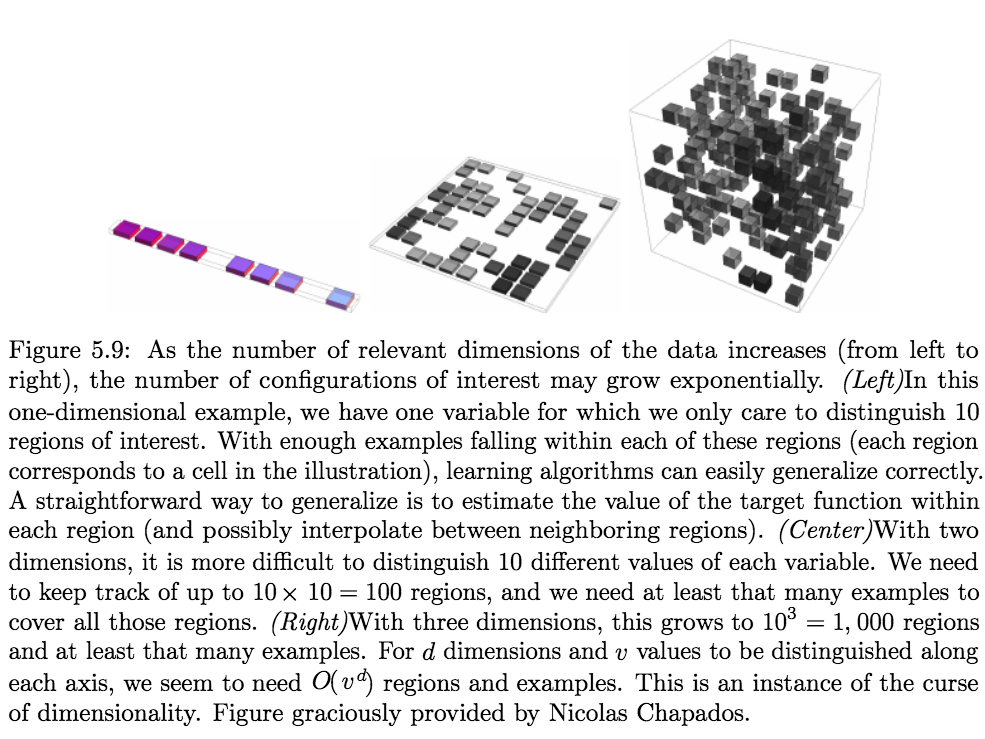
- Common Theme - Sparsity: When the dimensionality increases, the volume of the space increases so fast that the available data become sparse.
- Sparsity and Statistical Significance: This sparsity is problematic for any method that requires statistical significance. In order to obtain a statistically sound and reliable result, the amount of data needed to support the result often grows exponentially with the dimensionality.
- Sparsity and Clustering: Also, organizing and searching data often relies on detecting areas where objects form groups with similar properties (clustering); in high dimensional data, however, all objects appear to be sparse and dissimilar in many ways, which prevents common data organization strategies from being efficient.
- Statistical Challenge: the number of possible configurations of \(x\) is much larger than the number of training examples
- Stastical Sampling: The sampling density is proportional to \(N^{1/p}\), where \(p\) is the dimension of the input space and \(N\) is the sample size. Thus, if \(N_1 = 100\) represents a dense sample for a single input problem, then \(N_{10} = 100^{10}\) is the sample size required for the same sampling density with \(10\) inputs. Thus in high dimensions all feasible training samples sparsely populate the input space.
- Further Reading
- How to deal with curse of dimensionality?
- Feature Selection
- Feature Extraction
- Describe how to initialize a NN and any concerns w/ reasons:
- Don’t initialize the weights to Zero. The symmetry of hidden units results in a similar computation for each hidden unit, making all the rows of the weight matrix to be equal (by induction).
- It’s OK to initialize the bias term to zero.
- Describe the difference between Learning and Optimization in ML:
- The problem of Reducing the training error on the training set is one of optimization.
- The problem of Reducing the training error, as well as, the generalization (test) error is one of learning.
- List the 12 Standard Tasks in ML:
Answer- Clustering
- Forecasting
- Dimension reduction
- Sequence Labeling
- What is the difference between inductive and deductive learning?
- Inductive learning is the process of using observations to draw conclusions
- It is a method of reasoning in which the premises are viewed as supplying some evidence for the truth of the conclusion.
- It goes from specific to general (“bottom-up logic”).
- The truth of the conclusion of an inductive argument may be probable, based upon the evidence given.
- Deductive learning is the process of using conclusions to form observations.
- It is the process of reasoning from one or more statements (premises) to reach a logically certain conclusion.
- It goes from general to specific (“top-down logic”).
- The conclusions reached (“observations”) are necessarily True.
- Inductive learning is the process of using observations to draw conclusions
Statistical Learning Theory
- Define Statistical Learning Theory:
It is a framework for machine learning drawing from the fields of statistics and functional analysis that allows us, under certain assumptions, to study the question:How can we affect performance on the test set when we can only observe the training set?
It is a statistical approach to Computational Learning Theory.
- What assumptions are made by the theory?
- The training and test data are generated by an unknown data generating distribution (over the product space \(Z = X \times Y\), denoted: \(p_{\text{data}}(z) = p(x,y)\)) called the data-generating process.
- The i.i.d assumptions:
- The data-points in each dataset are independent from each other
- The training and testing are both identically distributed (drawn from the same distribution)
- Define the i.i.d assumptions?
A collection of random variables is independent and identically distributed if each random variable has the same probability distribution as the others and all are mutually independent. - Why assume a joint probability distribution \(p(x,y)\)?
Note that the assumption of a joint probability distribution allows us to model uncertainty in predictions (e.g. from noise in data) because \({\displaystyle y}\) is not a deterministic function of \({\displaystyle x}\), but rather a random variable with conditional distribution \({\displaystyle P(y|x)}\) for a fixed \({\displaystyle x}\). - Why do we need to model \(y\) as a target-distribution and not a target-function?
The ‘Target Function’ is not always a function because two ‘identical’ input points can be mapped to two different outputs (i.e. they have different labels).
- Give the Formal Definition of SLT:
- The Definitions:
- \(X\): \(\:\) Input (vector) Space
- \(Y\): \(\:\) Output (vector) Space
- \(Z = X \times Y\): \(\:\) Product space of (input, output) pairs
- \(n\): \(\:\) number of data points
- \(S = \left\{\left(\vec{x}_{1}, y_{1}\right), \ldots,\left(\vec{x}_{n}, y_{n}\right)\right\}=\left\{\vec{z}_{1}, \ldots, \vec{z}_{n}\right\}\): \(\:\) the training set
- \(\mathcal{H} = f : X \rightarrow Y\): \(\:\) the hypothesis space of all functions
- \(V(f(\vec{x}), y)\): \(\:\) an error/loss function
- The Assumptions:
- The training and testing sets are generated by an unknown data-generating distribution function (over \(Z\), denoted: \(p_{\text{data}} = p(z) = p(x,y)\)) called the data-generation process.
- The i.i.d assumptions:
- The examples in each dataset are generated independently from each other
- Both datasets are identically distributed
- The Inference Problem:
Find a function \(f : X \rightarrow Y\) such that \(f(\vec{x}) \sim y\). - The Expected Risk:
It is the overall average risk over the entire (data) probability-distribution:$$I[f] = \mathbf{E}[V(f(\vec{x}), y)]=\int_{X \times Y} V(f(\vec{x}), y) p(\vec{x}, y) d \vec{x} d y$$
- The Target Function:
It is the best possible function \(f\) that can be chosen, and is given by:$$f = \inf_{h \in \mathcal{H}} I[h]$$
- The Empirical Risk:
It is a proxy measure to the expected risk based on the training set. It is necessary since the probability distribution \(p(\vec{x}, y)\) is unknown.$$I_{S}[f]=\frac{1}{n} \sum_{i=1}^{n} V\left(f\left(\vec{x}_{i}\right), y_{i}\right)$$
- The Definitions:
-
Define Empirical Risk Minimization:
It is a (learning) principle in statistical learning theory that is based on approximating the Expected/True Risk (Generalization Error) by measuring the Empirical Risk (Training Error); i.e. the performance on the training-data.A learning algorithm that chooses the function \(f_S\) which minimizes the empirical risk is called Empirical Risk Minimization:
$$R_{\text{emp}} = I_S[f] = \dfrac{1}{n} \sum_{i=1}^n V(f(\vec{x}_ i, y_i))$$
$$f_{S} = \hat{h} = \arg \min _{h \in \mathcal{H}} R_{\mathrm{emp}}(h)$$
- What is the Complexity of ERM?
NP-Hard for classification with \(0-1\) loss function, even for linear classifiers- It can be solved efficiently when the minimal empirical risk is ZERO; i.e. the data is linearly separable
- How do you Cope with the Complexity?
- Employ a convex approximation to the \(0-1\) loss: Hinge, SVM etc.
- Imposing assumptions on the data-generating distribution thus, stop being an agnostic learning algorithm
- Definitions:
- Generalization:
The ability to do well on previously unobserved data:$$I[f] \approx I_S[f]$$
“Good” generalization is achieved when the empirical risk approximates the expected risk well.
-
Generalization Error:
AKA: Expected Risk, Out-of-sample Error, \(E_{\text{out}}\)
It is a measure of how accurately an algorithm is able to predict outcome values for previously unseen data defined as the expected value of the error on a new input, measured w.r.t. the data-generating probability distribution. - Generalization Gap:
It is a measure of how accurately an algorithm is able to predict outcome values for previously unseen data, defined as the difference between the expected risk and empirical risk:$$G =I\left[f_{n}\right]-I_{S}\left[f_{n}\right]$$
- Computing the Generalization Gap:
Since the empirical risk/generalization error \(I[f_n]\) cannot be computed for an unknown distribution, the generalization gap cannot be computed either. - What is the goal of SLT in the context of the Generalization Gap given that it can’t be computed?
Instead, the goal of SLT is to bound/characterize the gap in probability:$$P_{G}=P\left(I\left[f_{n}\right]-I_{S}\left[f_{n}\right] \leq \epsilon\right) \geq 1-\delta_{n}$$
I.E. goal is to characterize the probability \(1- \delta_n\) that the generalization gap is less than some error bound \(\epsilon\) (known as the learning rate)
- Computing the Generalization Gap:
- Achieving (“good”) Generalization:
An algorithm is said to generalize when the expected risk is well approximated by the empirical risk:$$I\left[f_{n}\right] \approx I_{S}\left[f_{n}\right]$$
Equivalently:
$$E_{\text {out}}(g) \approx E_{\text {in}}(g)$$
I.E. when the generalization gap approaches zero in the limit of data-points:
$$\lim _{n \rightarrow \infty} G_{n}=\lim _{n \rightarrow \infty} I\left[f_{n}\right]-I_{S}\left[f_{n}\right]=0$$
- Empirical Distribution:
AKA: Data-Generating Distribution
is the discrete, uniform, joint distribution \(p_{\text{data}} = p(x,y)\) over the sample points.
- Generalization:
- Describe the difference between Learning and Optimization in ML:
- Optimization: is concerned with the problem of reducing the training error on the training set
- Learning: is concerned with the problem of reducing the training error, as well as, the generalization (test) error
- Describe the difference between Generalization and Learning in ML:
- Generalization guarantee: tells us that it is likely that the following condition holds:
$$E_{\mathrm{out}}(\hat{h}) \approx E_{\mathrm{in}}(\hat{h})$$
I.E. that the empirical error tracks/approximates the expected/generalization error well.
- Learning: corresponds to the condition that \(\hat{h} \approx f\) the chosen hypothesis approximates the target function well, which in-turn corresponds to the condition:
$$E_{\mathrm{out}}(\hat{h}) \approx 0$$
- Generalization guarantee: tells us that it is likely that the following condition holds:
- How to achieve Learning?
To achieve learning we need to achieve the condition \(E_{\mathrm{out}}(\hat{h}) \approx 0\), which we do by:- \(E_{\mathrm{out}}(\hat{h}) \approx E_{\mathrm{in}}(\hat{h})\)
A theoretical result achieved through Hoeffding Inequality - \(E_{\mathrm{in}}(\hat{h}) \approx 0\)
A practical result of Empirical Error Minimization
- \(E_{\mathrm{out}}(\hat{h}) \approx E_{\mathrm{in}}(\hat{h})\)
- What does the (VC) Learning Theory Achieve?
- Characterizing the feasibility of learning for infinite hypotheses
- Characterizing the Approximation-Generalization Tradeoff
- Why do we need the probabilistic framework?
- What is the Approximation-Generalization Tradeoff:
It is a tradeoff between (1) How well we can approximate the target function \(f \:\:\) and (2) How well we can generalize to unseen data.
Given the goal: Small \(E_{\text{out}}\), good approximation of \(f\) out of sample (not in-sample).
The tradeoff is characterized by the complexity of the hypothesis space \(\mathcal{H}\):- More Complex \(\mathcal{H}\): Better chance of approximating \(f\)
- Less Complex \(\mathcal{H}\): Better chance of generalizing out-of-sample
- What are the factors determining how well an ML-algo will perform?
- Ability to Approximate \(f\) well, in-sample | Make the training error small &
- Decrease the gap between \(E_{\text{in}}\) and \(E_{\text{out}}\) | Make gap between training and test error small
- Define the following and their usage/application & how they relate to each other:
- Underfitting:
Occurs when the model cannot fit the training data well; high \(E_{\text{in}}\). - Overfitting:
Occurs when the gap between the training error and test error is too large. - Capacity:
a models ability to fit a high variety of functions (complexity).
It allows us to control the amount of overfitting and underfitting- Models with Low-Capacity:
Underfitting. High-Bias. Struggle to fit training-data. - Models with High-Capacity:
Overfitting. High-Variance. Memorizes noise.
- Models with Low-Capacity:
- Hypothesis Space:
The set of functions that the learning algorithm is allowed to select as being the target function.
Allows us to control the capacity of a model. - VC-Dimension:
The largest possible value of \(m\) for which there exists a training set of \(m\) different points that the classifier can label arbitrarily.
Quantifies a models capacity.- What does it measure?
Measures the capacity of a binary classifier.
- What does it measure?
- Graph the relation between Error, and Capacity in the ctxt of (Underfitting, Overfitting, Training Error, Generalization Err, and Generalization Gap):
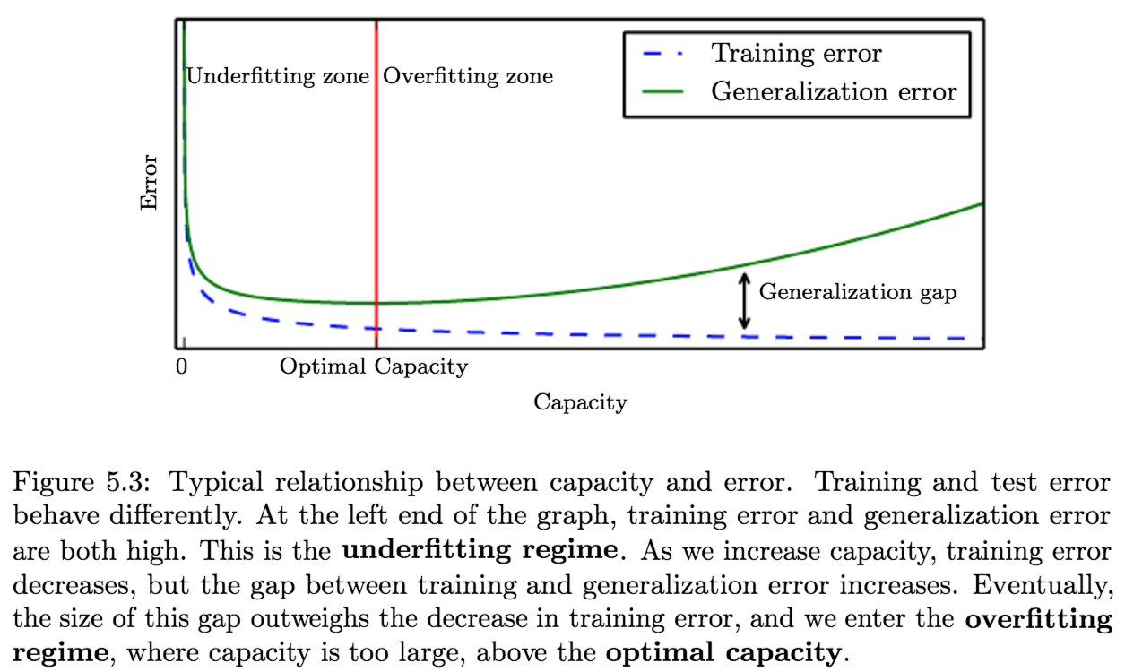
- Underfitting:
- What is the most important result in SLT that show that learning is feasible?
Shows that the discrepancy between training error and generalization error is bounded above by a quantity that grows as the model capacity grows but shrinks as the number of training examples increases.
Bias-Variance Decomposition Theory
- What is the Bias-Variance Decomposition Theory:
It is an approach for the quantification of the Approximation-Generalization Tradeoff. - What are the Assumptions made by the theory?
- Analysis is done over the entire data-distribution
- Real-Valued inputs, targets (can be extended)
- Target function \(f\) is known
- Uses MSE (can be extended)
- What is the question that the theory tries to answer? What assumption is important? How do you achieve the answer/goal?
- “How can \(\mathcal{H}\) approximate \(f\) overall? not just on our sample/training-data.”.
- We assume that the target function \(f\) is known.
- By taking the expectation over all possible realization of \(N\) data-points.
- What is the Bias-Variance Decomposition:
It is the decomposition of the expected error as a sum of three concepts: bias, variance and irreducible error, each quantifying an aspect of the error. - Define each term w.r.t. source of the error:
- Bias: the error from the erroneous/simplifying assumptions in the learning algorithm
- Variance: the error from sensitivity to small fluctuations in the training set
- Irreducible Error: the error resulting from the noise in the problem itself
- What does each of the following measure (error in)? Describe this measured quantity in words, mathematically. Describe Bias&Variance in Words as a question statement. Give their AKA in statistics.
- Bias:
- AKA: Approximation Error
- Measures the error in approximating the target function with the best possible hypothesis in \(\mathcal{H}\)
- The expected deviation from the true value of the function (or parameter)
- How well can \(\mathcal{H}\) approximate the target function \(f\)
- Variance:
- AKA: Estimation Error
- Measures the error in estimating the best possible hypothesis in \(\mathcal{H}\) with a particular hypothesis resulting from a specific training-set
- The deviation from the expected estimator value that any particular sampling of the data is likely to cause
- How well can we zoom in on a good \(h \in \mathcal{H}\)
- Irreducible Error: measures the inherent noise in the target \(y\)
- Bias:
- Give the Formal Definition of the Decomposition (Formula):
Given any hypothesis \(\hat{f} = g^{\mathcal{D}}\) we select, we can decompose its expected risk on an unseen sample \(x\) as:$$\mathbb{E}\left[(y-\hat{f}(x))^{2}\right]=(\operatorname{Bias}[\hat{f}(x)])^{2}+\operatorname{Var}[\hat{f}(x)]+\sigma^{2}$$
Where:
- Bias:
$$\operatorname{Bias}[\hat{f}(x)] = \mathbb{E}[\hat{f}(x)] - f(x)$$
- Variance:
$$\operatorname{Var}[\hat{f}(x)] = \mathbb{E}\left[(\hat{f}(x))^2\right] - \mathbb{E}\left[\hat{f}(x)\right]^2$$
- What is the Expectation over?
The expectation is over all different samplings of the data \(\mathcal{D}\)
- Bias:
- Define the Bias-Variance Tradeoff:
It is the property of a set of predictive models whereby, models with a lower bias have a higher variance and vice-versa.- Effects of Bias:
- High Bias: simple models \(\rightarrow\) underfitting
- Low Bias: complex models \(\rightarrow\) overfitting
- Effects of Variance:
- High Variance: complex models \(\rightarrow\) overfitting
- Low Variance: simple models \(\rightarrow\) underfitting
- Draw the Graph of the Tradeoff (wrt model capacity):
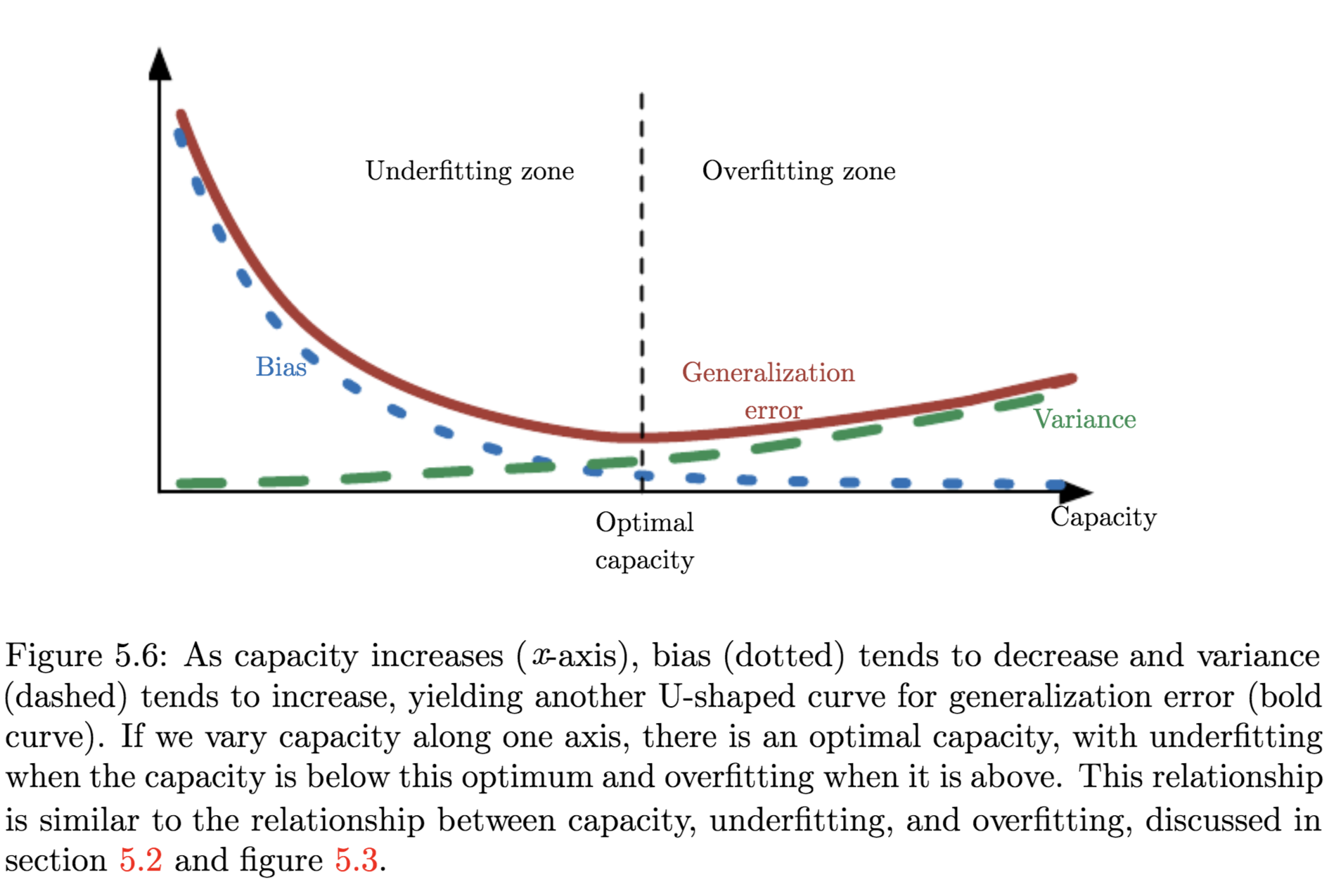
- Effects of Bias:
- Derive the Bias-Variance Decomposition with explanations:
$${\displaystyle {\begin{aligned}\mathbb{E}_{\mathcal{D}} {\big [}I[g^{(\mathcal{D})}]{\big ]}&=\mathbb{E}_{\mathcal{D}} {\big [}\mathbb{E}_{x}{\big [}(g^{(\mathcal{D})}-y)^{2}{\big ]}{\big ]}\\ &=\mathbb{E}_{x} {\big [}\mathbb{E}_{\mathcal{D}}{\big [}(g^{(\mathcal{D})}-y)^{2}{\big ]}{\big ]}\\ &=\mathbb{E}_{x}{\big [}\mathbb{E}_{\mathcal{D}}{\big [}(g^{(\mathcal{D})}- f -\varepsilon)^{2}{\big ]}{\big ]} \\&=\mathbb{E}_{x}{\big [}\mathbb{E}_{\mathcal{D}} {\big [}(f+\varepsilon -g^{(\mathcal{D})}+\bar{g}-\bar{g})^{2}{\big ]}{\big ]}\\ &=\mathbb{E}_{x}{\big [}\mathbb{E}_{\mathcal{D}} {\big [}(\bar{g}-f)^{2}{\big ]}+\mathbb{E}_{\mathcal{D}} [\varepsilon ^{2}]+\mathbb{E}_{\mathcal{D}} {\big [}(g^{(\mathcal{D})} - \bar{g})^{2}{\big ]}+2\: \mathbb{E}_{\mathcal{D}} {\big [}(\bar{g}-f)\varepsilon {\big ]}+2\: \mathbb{E}_{\mathcal{D}} {\big [}\varepsilon (g^{(\mathcal{D})}-\bar{g}){\big ]}+2\: \mathbb{E}_{\mathcal{D}} {\big [}(g^{(\mathcal{D})} - \bar{g})(\bar{g}-f){\big ]}{\big ]}\\ &=\mathbb{E}_{x}{\big [}(\bar{g}-f)^{2}+\mathbb{E}_{\mathcal{D}} [\varepsilon ^{2}]+\mathbb{E}_{\mathcal{D}} {\big [}(g^{(\mathcal{D})} - \bar{g})^{2}{\big ]}+2(\bar{g}-f)\mathbb{E}_{\mathcal{D}} [\varepsilon ]\: +2\: \mathbb{E}_{\mathcal{D}} [\varepsilon ]\: \mathbb{E}_{\mathcal{D}} {\big [}g^{(\mathcal{D})}-\bar{g}{\big ]}+2\: \mathbb{E}_{\mathcal{D}} {\big [}g^{(\mathcal{D})}-\bar{g}{\big ]}(\bar{g}-f){\big ]}\\ &=\mathbb{E}_{x}{\big [}(\bar{g}-f)^{2}+\mathbb{E}_{\mathcal{D}} [\varepsilon ^{2}]+\mathbb{E}_{\mathcal{D}} {\big [}(g^{(\mathcal{D})} - \bar{g})^{2}{\big ]}{\big ]}\\ &=\mathbb{E}_{x}{\big [}(\bar{g}-f)^{2}+\operatorname {Var} [y]+\operatorname {Var} {\big [}g^{(\mathcal{D})}{\big ]}{\big ]}\\ &=\mathbb{E}_{x}{\big [}\operatorname {Bias} [g^{(\mathcal{D})}]^{2}+\operatorname {Var} [y]+\operatorname {Var} {\big [}g^{(\mathcal{D})}{\big ]}{\big ]}\\ &=\mathbb{E}_{x}{\big [}\operatorname {Bias} [g^{(\mathcal{D})}]^{2}+\sigma ^{2}+\operatorname {Var} {\big [}g^{(\mathcal{D})}{\big ]}{\big ]}\\\end{aligned}}}$$
where:
\(\overline{g}(\mathbf{x})=\mathbb{E}_{\mathcal{D}}\left[g^{(\mathcal{D})}(\mathbf{x})\right]\) is the average hypothesis over all realization of \(N\) data-points \(\mathcal{D}_ i\), and \({\displaystyle \varepsilon }\) and \({\displaystyle {\hat {f}}} = g^{(\mathcal{D})}\) are independent. - What are the key Takeaways from the Tradeoff?
Match the “Model Capacity/Complexity” to the “Data Resources”, NOT to the Target Complexity. - What are the most common ways to negotiate the Tradeoff?
- Cross-Validation
- MSE of the Estimates
- How does the decomposition relate to Classification?
A similar decomposition exists for:- Classification with \(0-1\) loss
- Probabilistic Classification with MSE
- Increasing/Decreasing Bias&Variance:
- Adding Good Feature:
- Decrease Bias
- Adding Bad Feature:
- No effect
- Adding ANY Feature:
- Increase Variance
- Adding more Data:
- Decrease Variance
- May decrease Bias (if \(f \in \mathcal{H}\) | \(h\) can fit \(f\) exactly)
- Noise in Test Set:
- Affects Only Irreducible Err
- Noise in Training Set:
- Affects Bias and Variance
- Dimensionality Reduction:
- Decrease Variance
- Feature Selection:
- Decrease Variance
- Regularization:
- Increase Bias
- Decrease Variance
- Increasing # of Hidden Units in ANNs:
- Decrease Bias
- Increase Variance
- Increasing # of Hidden Layers in ANNs:
- Decrease Bias
- Increase Variance
- Increasing \(k\) in K-NN:
- Increase Bias
- Decrease Variance
- Increasing Depth in Decision-Trees:
- Increase Variance
- Boosting:
- Decrease Bias
- Bagging:
- Decrease Variance
- Adding Good Feature:
Activation Functions
- Describe the Desirable Properties for activation functions:
- Non-Linearity:
When the activation function is non-linear, then a two-layer neural network can be proven to be a universal function approximator. The identity activation function does not satisfy this property. When multiple layers use the identity activation function, the entire network is equivalent to a single-layer model. - Range:
When the range of the activation function is finite, gradient-based training methods tend to be more stable, because pattern presentations significantly affect only limited weights. When the range is infinite, training is generally more efficient because pattern presentations significantly affect most of the weights. In the latter case, smaller learning rates are typically necessary. - Continuously Differentiable:
This property is desirable for enabling gradient-based optimization methods. The binary step activation function is not differentiable at 0, and it differentiates to 0 for all other values, so gradient-based methods can make no progress with it. - Monotonicity:
When the activation function is monotonic, the error surface associated with a single-layer model is guaranteed to be convex. - Smoothness with Monotonic Derivatives:
These have been shown to generalize better in some cases. - Approximating Identity near Origin:
Equivalent to \({\displaystyle f(0)=0}\) and \({\displaystyle f'(0)=1}\), and \({\displaystyle f'}\) is continuous at \(0\).
When activation functions have this property, the neural network will learn efficiently when its weights are initialized with small random values. When the activation function does not approximate identity near the origin, special care must be used when initializing the weights. - Zero-Centered Range:
Has effects of centering the data (zero mean) by centering the activations. Makes learning easier.
- Non-Linearity:
- Range:
- Continuously Differentiable:
- Monotonicity:
- Smoothness with Monotonic Derivatives:
- Approximating Identity near Origin:
- Zero-Centered Range:
- Non-Linearity:
- Describe the NON-Desirable Properties for activation functions:
- Saturation:
An activation functions output, with finite range, may saturate near its tail or head (e.g. \(\{0, 1\}\) for sigmoid). This leads to a problem called vanishing gradient. - Vanishing Gradients:
Happens when the gradient of an activation function is very small/zero. This usually happens when the activation function saturates at either of its tails.
The chain-rule will multiply the local gradient (of activation function) with the whole objective. Thus, when gradient is small/zero, it will “kill” the gradient \(\rightarrow\) no signal will flow through the neuron to its weights or to its data.
Slows/Stops learning completely. - Range Not Zero-Centered:
This is undesirable since neurons in later layers of processing in a Neural Network would be receiving data that is not zero-centered. This has implications on the dynamics during gradient descent, because if the data coming into a neuron is always positive (e.g. \(x>0\) elementwise in \(f=w^Tx+b\)), then the gradient on the weights \(w\) will during backpropagation become either all be positive, or all negative (depending on the gradient of the whole expression \(f\)). This could introduce undesirable zig-zagging dynamics in the gradient updates for the weights. However, notice that once these gradients are added up across a batch of data the final update for the weights can have variable signs, somewhat mitigating this issue. Therefore, this is an inconvenience but it has less severe consequences compared to the saturated activation problem above.
Makes optimization harder.
- Saturation:
- Vanishing Gradients:
- Range Not Zero-Centered:
- Saturation:
- List the different activation functions used in ML?
Identity, Sigmoid, Tanh, ReLU, L-ReLU, ELU, SoftPlus
Names, Definitions, Properties (pros&cons), Derivatives, Applications, pros/cons:- Sigmoid:
$$S(z)=\frac{1}{1+e^{-z}} \\ S^{\prime}(z)=S(z) \cdot(1-S(z))$$
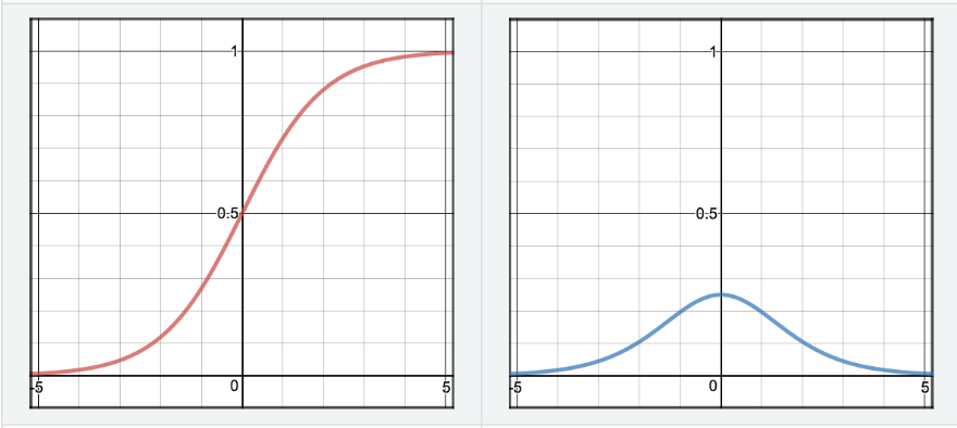
- Properties:
Never use as activation, use as an output unit for binary classification.- Pros:
- Has a nice interpretation as the firing rate of a neuron
- Cons:
- They Saturate and kill gradients \(\rightarrow\) Gives rise to vanishing gradients \(\rightarrow\) Stop Learning
- Happens when initialization weights are too large
- or sloppy with data preprocessing
- Neurons Activation saturates at either tail of \(0\) or \(1\)
- Output NOT Zero-Centered \(\rightarrow\) Gradient updates go too far in different directions \(\rightarrow\) makes optimization harder
- The local gradient \((z * (1-z))\) achieves maximum at \(0.25\), when \(z = 0.5\). \(\rightarrow\) very time the gradient signal flows through a sigmoid gate, its magnitude always diminishes by one quarter (or more) \(\rightarrow\) with basic SGD, the lower layers of a network train much slower than the higher one
- They Saturate and kill gradients \(\rightarrow\) Gives rise to vanishing gradients \(\rightarrow\) Stop Learning
- Pros:
- Properties:
- Tanh:
$$\tanh (z)=\frac{e^{z}-e^{-z}}{e^{z}+e^{-z}} \\ \tanh ^{\prime}(z)=1-\tanh (z)^{2}$$
Properties:
Strictly superior to Sigmoid (scaled version of sigmoid | stronger gradient). Good for activation.- Pros:
- Zero Mean/Centered
- Cons:
- They Saturate and kill gradients \(\rightarrow\) Gives rise to vanishing gradients \(\rightarrow\) Stop Learning
- Pros:
- Relu:
$$R(z)=\left\{\begin{array}{cc}{z} & {z>0} \\ {0} & {z<=0}\end{array}\right\} \\ R^{\prime}(z)=\left\{\begin{array}{ll}{1} & {z>0} \\ {0} & {z<0}\end{array}\right\}$$
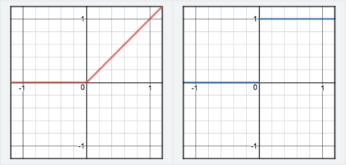
Properties:
The best for activation (Better gradients).- Pros:
- Non-saturation of gradients which accelerates convergence of SGD
- Sparsity effects and induced regularization. discussion
- Not computationally expensive
- Cons:
- ReLU not zero-centered problem:
The problem that ReLU is not zero-centered can be solved/mitigated by using batch normalization, which normalizes the signal before activation:From paper: We add the BN transform immediately before the nonlinearity, by normalizing \(x = Wu + b\); normalizing it is likely to produce activations with a stable distribution.
- Dying ReLUs (Dead Neurons):
If a neuron gets clamped to zero in the forward pass (it doesn’t “fire” / \(x<0\)), then its weights will get zero gradient. Thus, if a ReLU neuron is unfortunately initialized such that it never fires, or if a neuron’s weights ever get knocked off with a large update during training into this regime (usually as a symptom of aggressive learning rates), then this neuron will remain permanently dead. - Infinite Range:
Can blow up the activation.
- ReLU not zero-centered problem:
- Pros:
- Leaky Relu:
$$R(z)=\left\{\begin{array}{cc}{z} & {z>0} \\ {\alpha z} & {z<=0}\end{array}\right\} \\ R^{\prime}(z)=\left\{\begin{array}{ll}{1} & {z>0} \\ {\alpha} & {z<0}\end{array}\right\}$$
Properties:
Sometimes useful. Worth trying.- Pros:
- Leaky ReLUs are one attempt to fix the “dying ReLU” problem by having a small negative slope (of 0.01, or so).
- Cons:
The consistency of the benefit across tasks is presently unclear.
- Pros:
- Sigmoid:
- Fill in the following table:
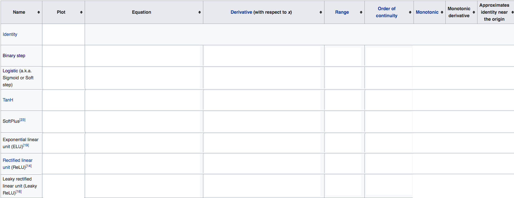
- Tanh VS Sigmoid for activation?
Tanh > Sigmoid - ReLU:
$$R(z)=\left\{\begin{array}{cc}{z} & {z>0} \\ {0} & {z<=0}\end{array}\right\} \\ R^{\prime}(z)=\left\{\begin{array}{ll}{1} & {z>0} \\ {0} & {z<0}\end{array}\right\}$$
Properties:
The best for activation (Better gradients).- Pros:
- Non-saturation of gradients which accelerates convergence of SGD
- Sparsity effects and induced regularization. discussion
- Not computationally expensive
- Cons:
- ReLU not zero-centered problem:
The problem that ReLU is not zero-centered can be solved/mitigated by using batch normalization, which normalizes the signal before activation:From paper: We add the BN transform immediately before the nonlinearity, by normalizing \(x = Wu + b\); normalizing it is likely to produce activations with a stable distribution.
- Dying ReLUs (Dead Neurons):
If a neuron gets clamped to zero in the forward pass (it doesn’t “fire” / \(x<0\)), then its weights will get zero gradient. Thus, if a ReLU neuron is unfortunately initialized such that it never fires, or if a neuron’s weights ever get knocked off with a large update during training into this regime (usually as a symptom of aggressive learning rates), then this neuron will remain permanently dead. - Infinite Range:
Can blow up the activation.
- ReLU not zero-centered problem:
- What makes it superior/advantageous?
Larger Derivatives. - What problems does it have?
- What solution do we have to mitigate the problem?
Batch Normalization.
- What solution do we have to mitigate the problem?
- Pros:
- Compute the derivatives of all activation functions:
- Graph all activation functions and their derivatives:
Kernels
- Define “Local Kernel” and give an analogy to describe it:
- Write the following kernels:
- Polynomial Kernel of degree, up to, \(d\):
- Gaussian Kernel:
- Sigmoid Kernel:
- Polynomial Kernel of degree, exactly, \(d\):
Math
- What is a metric?
A Metric (distance function) \(d\) is a function that defines a distance between each pair of elements of a set \(X\).
A Metric induces a topology on a set; BUT, not all topologies can be generated by a metric.
Mathematically, it is a function:
\({\displaystyle d:X\times X\to [0,\infty )},\)
that must satisfy the following properties:- \({\displaystyle d(x,y)\geq 0}\) \(\:\:\:\:\:\:\:\) non-negativity or separation axiom
- \({\displaystyle d(x,y)=0\Leftrightarrow x=y}\) \(\:\:\:\:\:\:\:\) identity of indiscernibles
- \({\displaystyle d(x,y)=d(y,x)}\) \(\:\:\:\:\:\:\:\) symmetry
- \({\displaystyle d(x,z)\leq d(x,y)+d(y,z)}\) \(\:\:\:\:\:\:\:\) subadditivity or triangle inequality
The first condition is implied by the others.
Metric
- Describe Binary Relations and their Properties?
A binary relation on a set \(A\) is a set of ordered pairs of elements of \(A\). In other words, it is a subset of the Cartesian product \(A^2 = A ×A\).
The number of binary relations on a set of \(N\) elements is \(= 2^{N^2}\) Examples:- “is greater than”
- “is equal to”
- A function \(f(x)\)
Properties: (for a relation \(R\) and set \(X\)) - Reflexive: for all \(x\) in \(X\) it holds that \(xRx\)
- Symmetric: for all \(x\) and \(y\) in \(X\) it holds that if \(xRy\) then \(yRx\)
- Transitive: for all \(x\), \(y\) and \(z\) in \(X\) it holds that if \(xRy\) and \(yRz\) then \(xRz\)
answer
- Formulas:
- Set theory:
- Number of subsets of a set of \(N\) elements:
\(= 2^N\) - Number of pairs \((a,b)\) of a set of N elements:
\(= N^2\)
- Number of subsets of a set of \(N\) elements:
- Binomial Theorem:
$$(x+y)^{n}=\sum_{k=0}^{n}{n \choose k}x^{n-k}y^{k}=\sum_{k=0}^{n}{n \choose k}x^{k}y^{n-k} \\={n \choose 0}x^{n}y^{0}+{n \choose 1}x^{n-1}y^{1}+{n \choose 2}x^{n-2}y^{2}+\cdots +{n \choose n-1}x^{1}y^{n-1}+{n \choose n}x^{0}y^{n},$$
- Binomial Coefficient:
$${\binom {n}{k}}={\frac {n!}{k!(n-k)!}} = N \text{choose} k = N \text{choose} (n-k)$$
- Expansion of \(x^n - y^n =\)
$$x^n - y^n = (x-y)(x^{n-1} + x^{n-2} y + ... + x y^{n-2} + y^{n-1})$$
- Number of ways to partition \(N\) data points into \(k\) clusters:
- Number of pairs (e.g. \((a,b)\)) of a set of \(N\) elements \(= N^2\)
- There are at most \(k^N\) ways to partition \(N\) data points into \(k\) clusters - there are \(N\) choose \(k\) clusters, precisely
- \(\log_x(y) =\)
$$\log_x(y) = \dfrac{\ln(y)}{\ln(x)}$$
- The length of a vector \(\mathbf{x}\) along a direction (projection):
- Along a unit-length vector \(\hat{\mathbf{w}}\):
\(\text{comp}_ {\hat{\mathbf{w}}}(\mathbf{x}) = \hat{\mathbf{w}}^T\mathbf{x}\) - Along an unnormalized vector \(\mathbf{w}\):
\(\text{comp}_ {\mathbf{w}}(\mathbf{x}) = \dfrac{1}{\|\mathbf{w}\|} \mathbf{w}^T\mathbf{x}\)
- Along a unit-length vector \(\hat{\mathbf{w}}\):
- \(\sum_{i=1}^{n} 2^{i}=\)
\(\sum_{i=1}^{n} 2^{i}=2^{n+1}-2\)
- Set theory:
- List 6 proof methods:
- Direct Proof
- Mathematical Induction
- Strong Induction
- Infinite Descent
- Contradiction
- Contraposition (\((p \implies q) \iff (!q \implies !p)\))
- Construction
- Combinatorial
- Exhaustion
- Non-Constructive proof (existence proofs) answer
- Important Formulas
- Projection \(\tilde{\mathbf{x}}\) of a vector \(\mathbf{x}\) onto another vector \(\mathbf{u}\):
$$\tilde{\mathbf{x}} = \mathbf{x}\cdot \dfrac{\mathbf{u}}{\|\mathbf{u}\|_2} \mathbf{u}$$
- Projection \(\tilde{\mathbf{x}}\) of a vector \(\mathbf{x}\) onto another vector \(\mathbf{u}\):
Statistics
- ROC curve:
- Definition:
A receiver operating characteristic curve, or ROC curve, is a graphical plot that illustrates the diagnostic ability of a binary classifier system as its discrimination threshold is varied. - Purpose:
A way to quantify how good a binary classifier separates two classes. - How do you create the plot?
The ROC curve is created by plotting the true positive rate (TPR) against the false positive rate (FPR) at various threshold settings.
- \(\mathrm{TPR}=\frac{\mathrm{TP}}{\mathrm{P}}=\frac{\mathrm{TP}}{\mathrm{TP}+\mathrm{FN}}\)
- \(\mathrm{FPR}=\frac{\mathrm{FP}}{\mathrm{N}}=\frac{\mathrm{FP}}{\mathrm{FP}+\mathrm{TN}}\) - How to identify a good classifier:
A Good classifier has a ROC curve that is near the top-left diagonal (hugging it). - How to identify a bad classifier:
A Bad Classifier has a ROC curve that is close to the diagonal line. - What is its application in tuning the model?
It allows you to set the classification threshold:- You can minimize False-positive rate or maximize the True-Positive Rate
- Definition:
- AUC - AUROC:
- Definition:
When using normalized units, the area under the curve (often referred to as simply the AUC) is equal to the probability that a classifier will rank a randomly chosen positive instance higher than a randomly chosen negative one (assuming ‘positive’ ranks higher than ‘negative’). - Range:
Range \(= 0.5 - 1.0\), from poor to perfect, with an uninformative classifier yielding \(0.5\) - What does it measure:
It is a measure of aggregated classification performance. - Usage in ML:
For model comparison.
- Definition:
-
Define Statistical Efficiency (of an estimator)?
Essentially, a more efficient estimator, experiment, or test needs fewer observations than a less efficient one to achieve a given performance.
Efficiencies are often defined using the variance or mean square error as the measure of desirability.
An efficient estimator is also the minimum variance unbiased estimator (MVUE).- An Efficient Estimator has lower variance than an inefficient one
- The use of an inefficient estimator gives results equivalent to those obtainable from a subset of data; and is therefor, wasteful of data
-
Whats the difference between Errors and Residuals:
The Error of an observed value is the deviation of the observed value from the (unobservable) true value of a quantity of interest.The Residual of an observed value is the difference between the observed value and the estimated value of the quantity of interest.
- Compute the statistical errors and residuals of the univariate, normal distribution defined as \(X_{1}, \ldots, X_{n} \sim N\left(\mu, \sigma^{2}\right)\):
- Statistical Errors:
$$e_{i}=X_{i}-\mu$$
- Residuals:
$$r_{i}=X_{i}-\overline {X}$$
- Example in Univariate Distributions
- Statistical Errors:
- Compute the statistical errors and residuals of the univariate, normal distribution defined as \(X_{1}, \ldots, X_{n} \sim N\left(\mu, \sigma^{2}\right)\):
- What is a biased estimator?
We define the Bias of an estimator as:$$ \operatorname{bias}\left(\hat{\boldsymbol{\theta}}_{m}\right)=\mathbb{E}\left(\hat{\boldsymbol{\theta}}_{m}\right)-\boldsymbol{\theta} $$
A Biased Estimator is an estimator \(\hat{\boldsymbol{\theta}}_ {m}\) such that:
$$ \operatorname{bias}\left(\hat{\boldsymbol{\theta}}_ {m}\right) \geq 0$$
- Why would we prefer biased estimators in some cases?
Mainly, due to the Bias-Variance Decomposition. The MSE takes into account both the bias and the variance and sometimes the biased estimator might have a lower variance than the unbiased one, which results in a total decrease in the MSE.
- Why would we prefer biased estimators in some cases?
- What is the difference between “Probability” and “Likelihood”:
Probabilities are the areas under a fixed distribution
\(pr(\)data\(|\)distribution\()\)
i.e. probability of some data (left hand side) given a distribution (described by the right hand side)
Likelihoods are the y-axis values for fixed data points with distributions that can be moved..
\(L(\)distribution\(|\)observation/data\()\)
It is the likelihood of the parameter \(\theta\) for the data \(\mathcal{D}\).Likelihood is, basically, a specific probability that can only be calculated after the fact (of observing some outcomes). It is not normalized to \(1\) (it is not a probability). It is just a way to quantify how likely a set of observation is to occur given some distribution with some parameters; then you can manipulate the parameters to make the realization of the data more “likely” (it is precisely meant for that purpose of estimating the parameters); it is a function of the parameters.
Probability, on the other hand, is absolute for all possible outcomes. It is a function of the Data. - Estimators:
- Define:
A Point Estimator or statistic is any function of the data. - Formula:
$$\hat{\boldsymbol{\theta}}_{m}=g\left(\boldsymbol{x}^{(1)}, \ldots, \boldsymbol{x}^{(m)}\right)$$
- Whats a good estimator?
A good estimator is a function whose output is close to the true underlying \(\theta\) that generated the training data. - What are the Assumptions made regarding the estimated parameter:
We assume that the true \(\boldsymbol{\theta}\) is fixed, and that \(\hat{\boldsymbol{\theta}}\) is a function of the data, which is drawn from a random process, making \(\hat{\boldsymbol{\theta}}\) a random variable.
- Define:
- What is Function Estimation:
Function Estimation/Approximation refers to estimation of the relationship between input and target data.
I.E. We are trying to predict a variable \(y\) given an input vector \(x\), and we assume that there is a function \(f(x)\) that describes the approximate relationship between \(y\) and \(x\).
If we assume that: \(y = f(x) + \epsilon\), where \(\epsilon\) is the part of \(y\) that is not predictable from \(x\); then we are interested in approximating \(f\) with a model or estimate \(\hat{f}\).- Whats the relation between the Function Estimator \(\hat{f}\) and Point Estimator:
Function estimation is really just the same as estimating a parameter \(\boldsymbol{\theta}\); the function estimator \(\hat{f}\) is simply a point estimator in function space.
- Whats the relation between the Function Estimator \(\hat{f}\) and Point Estimator:
- Define “marginal likelihood” (wrt naive bayes):
Marginal likelihood is, the probability that the word ‘FREE’ is used in any message (not given any other condition?).
(Statistics) - MLE
- Clearly Define MLE and derive the final formula:
MLE is a method/principle from which we can derive specific functions that are good estimators for different models.
Likelihood in Parametric Models:
Suppose we have a parametric model \(\{p(y ; \theta) | \theta \in \Theta\}\) and a sample \(D=\left\{y_{1}, \ldots, y_{n}\right\}\):- The likelihood of parameter estimate \(\hat{\theta} \in \Theta\) for sample \(\mathcal{D}\) is:
$$\begin{aligned} {\displaystyle {\mathcal {L}}(\theta \,;\mathcal{D} )} &= p(\mathcal{D} ; \theta) \\&=\prod_{i=1}^{n} p\left(y_{i} ; \theta\right)\end{aligned}$$
- In practice, we prefer to work with the log-likelihood. Same maximum but
$$\log {\displaystyle {\mathcal {L}}(\theta \,;\mathcal{D} )}=\sum_{i=1}^{n} \log p\left(y_{i} ; \theta\right)$$
and sums are easier to work with than products.
MLE for Parametric Models:
The maximum likelihood estimator (MLE) for \(\theta\) in the (parametric) model \(\{p(y, \theta) | \theta \in \Theta\}\) is:$$\begin{aligned} \hat{\theta} &=\underset{\theta \in \Theta}{\arg \max } \log p(\mathcal{D}, \hat{\theta}) \\ &=\underset{\theta \in \Theta}{\arg \max } \sum_{i=1}^{n} \log p\left(y_{i} ; \theta\right) \end{aligned}$$
- Write MLE as an expectation wrt the Empirical Distribution:
Because the \(\text {arg max }\) does not change when we rescale the cost function, we can divide by \(m\) to obtain a version of the criterion that is expressed as an expectation with respect to the empirical distribution \(\hat{p}_ {\text {data}}\) defined by the training data:$${\displaystyle \boldsymbol{\theta}_{\mathrm{ML}}=\underset{\boldsymbol{\theta}}{\arg \max } \:\: \mathbb{E}_{\mathbf{x} \sim \hat{p} \text {data}} \log p_{\text {model}}(\boldsymbol{x} ; \boldsymbol{\theta})} \tag{5.59}$$
- Describe formally the relationship between MLE and the KL-divergence:
MLE as Minimizing KL-Divergence between the Empirical dist. and the model dist.:
We can interpret maximum likelihood estimation as minimizing the dissimilarity between the empirical distribution \(\hat{p}_ {\text {data}}\), defined by the training set, and the model distribution, with the degree of dissimilarity between the two measured by the KL divergence.- The KL-divergence is given by:
$${\displaystyle D_{\mathrm{KL}}\left(\hat{p}_{\text {data}} \| p_{\text {model}}\right)=\mathbb{E}_{\mathbf{x} \sim \hat{p}_{\text {data}}}\left[\log \hat{p}_{\text {data}}(\boldsymbol{x})-\log p_{\text {model}}(\boldsymbol{x})\right]} \tag{5.60}$$
The term on the left is a function only of the data-generating process, not the model. This means when we train the model to minimize the KL divergence, we need only minimize:
$${\displaystyle -\mathbb{E}_{\mathbf{x} \sim \hat{p}_{\text {data}}}\left[\log p_{\text {model}}(\boldsymbol{x})\right]} \tag{5.61}$$
which is of course the same as the maximization in equation \(5.59\).
- The KL-divergence is given by:
-
Extend the argument to show the link between MLE and Cross-Entropy. Give an example:
Minimizing this KL-divergence corresponds exactly to minimizing the cross-entropy between the distributions.
Any loss consisting of a negative log-likelihood is a cross-entropy between the empirical distribution defined by the training set and the probability distribution defined by model.
E.g. MSE is the cross-entropy between the empirical distribution and a Gaussian model.Maximum likelihood thus becomes minimization of the negative log-likelihood(NLL), or equivalently, minimization of the cross-entropy.
- How does MLE relate to the model distribution and the empirical distribution?
We can thus see maximum likelihood as an attempt to make the model distribution match the empirical distribution \(\hat{p} _ {\text {data}}\). - What is the intuition behind using MLE?
If I choose a hypothesis \(h\) underwhich the observed data is very plausible then the hypothesis is very likely. - What does MLE find/result in?
It finds the value of the parameter \(\theta\) that, if used (in the model) to generate the probability of the data, would make the data most “likely” to occur. - What kind of problem is MLE and how to solve for it?
It is an optimization problem that is solved by calculus for problems with closed-form solutions or with numerical methods (e.g. SGD). - How does it relate to SLT:
It corresponds to Empirical Risk Minimization. - Explain clearly why we maximize the natural log of the likelihood
- Numerical Stability: change products to sums
- The logarithm of a member of the family of exponential probability distributions (which includes the ubiquitous normal) is polynomial in the parameters (i.e. max-likelihood reduces to least-squares for normal distributions)
\(\log\left(\exp\left(-\frac{1}{2}x^2\right)\right) = -\frac{1}{2}x^2\) - The latter form is both more numerically stable and symbolically easier to differentiate than the former. It increases the dynamic range of the optimization algorithm (allowing it to work with extremely large or small values in the same way).
- The logarithm is a monotonic transformation that preserves the locations of the extrema (in particular, the estimated parameters in max-likelihood are identical for the original and the log-transformed formulation)
- Gradient methods generally work better optimizing \(log_p(x)\) than \(p(x)\) because the gradient of \(log_p(x)\) is generally more well-scaled. link
Justification: the gradient of the original term will include a \(e^{\vec{x}}\) multiplicative term that scales very quickly one way or another, requiring the step-size to equally scale/stretch in the opposite direction.
- The likelihood of parameter estimate \(\hat{\theta} \in \Theta\) for sample \(\mathcal{D}\) is:
Text-Classification | Classical
- List some Classification Methods:
- (Hand-Coded)Rules-Based Algorithms: use rules based on combinations of words or other features.
- Can have high accuracy if the rules are carefully refined and maintained by experts.
- However, building and maintaining these rules is very hard.
- Supervised Machine Learning: using an ML algorithm that trains on a training set of (document, class) elements to train a classifier.
- Types of Classifiers:
- Naive Bayes
- Logistic Regression
- SVMs
- K-NNs
- Types of Classifiers:
- (Hand-Coded)Rules-Based Algorithms: use rules based on combinations of words or other features.
- List some Applications of Txt Classification:
- Spam Filtering: discerning spam emails form legitimate emails.
- Email Routing: sending an email sento to a genral address to a specfic affress based on the topic.
- Language Identification: automatiacally determining the genre of a piece of text.
- Readibility Assessment__: determining the degree of readability of a piece of text.
- Sentiment Analysis: determining the general emotion/feeling/attitude of the author of a piece of text.
- Authorship Attribution: determining which author wrote which piece of text.
- Age/Gender Identification: determining the age and/or gender of the author of a piece of text.
NLP
- List some problems in NLP:
- Question Answering (QA)
- Information Extraction (IE)
- Sentiment Analysis
- Machine Translation (MT)
- Spam Detection
- Parts-of-Speech (POS) Tagging
- Named Entity Recognition (NER)
- Conference Resolution
- Word Sense Disambugation (WSD)
- Parsing
- Paraphrasing
- Summarization
- Dialog
- List the Solved Problems in NLP:
- Spam Detection
- Parts-of-Speech (POS) Tagging
- Named Entity Recognition (NER)
- List the “within reach” problems in NLP:
- Sentiment Analysis
- Conference Resolution
- Word Sense Disambugation (WSD)
- Parsing
- Machine Translation (MT)
- Information Extraction (IE)
- List the Open Problems in NLP:
- Question Answering (QA)
- Paraphrasing
- Summarization
- Dialog
- Why is NLP hard? List Issues:
- Non-Standard English: “Great Job @ahmed_badary! I luv u 2!! were SOO PROUD of dis.”
- Segmentation Issues: “New York-New Haven” vs “New-York New-Haven”
- Idioms: “dark horse”, “getting cold feet”, “losing face”
- Neologisms: “unfriend”, “retweet”, “google”, “bromance”
- World Knowledge: “Ahmed and Zach are brothers”, “Ahmed and Zach are fathers”
- Tricky Entity Names: “Where is Life of Pie playing tonight?”, “Let it be was a hit song!”
- Define:
- Morphology:
The study of words, how they are formed, and their relationship to other words in the same language. - Morphemes:
the small meaningful units that make up words. - Stems:
the core meaning-bearing units of words. - Affixes:
the bits and pieces that adhere to stems (often with grammatical functions). - Stemming:
is the process of reducing inflected (or sometimes derived) words to their word stem, base or root form.
The stem need not map to a valid root in the language. - Lemmatization:
reducing inflections or variant forms to base form.
- Morphology:
- Topic Modeling vs Document Classification:
- Text Classification is a form of supervised learning, hence the set of possible classes are known/defined in advance, and won’t change.
- Topic Modeling is a form of unsupervised learning (akin to clustering), so the set of possible topics are unknown apriori. They’re defined as part of generating the topic models.
Language Modeling
- What is a Language Model?
- List some Applications of LMs:
- Traditional LMs:
- How are they setup?
- What do they depend on?
- What is the Goal of the LM task? (in the ctxt of the problem setup)
- What assumptions are made by the problem setup? Why?
- What are the MLE Estimates for probabilities of the following:
- Bi-Grams:
$$p(w_2\vert w_1) = $$
- Tri-Grams:
$$p(w_3\vert w_1, w_2) = $$
- Bi-Grams:
- What are the issues w/ Traditional Approaches?
- What+How can we setup some NLP tasks as LM tasks:
- How does the LM task relate to Reasoning/AGI:
- Evaluating LM models:
- List the Loss Functions (+formula) used to evaluate LM models? Motivate each:
- Which application of LM modeling does each loss work best for?
- Why Cross-Entropy:
- Which setting it used for?
- Why Perplexity:
- Which setting used for?
- If no surprise, what is the perplexity?
- How does having a good LM relate to Information Theory?
- LM DATA:
- How does the fact that LM is a time-series prediction problem affect the way we need to train/test:
- How should we choose a subset of articles for testing:
- List three approaches to Parametrizing LMs:
- Describe “Count-Based N-gram Models”:
- What distributions do they capture?:
- Describe “Neural N-gram Models”:
- What do they replace the captured distribution with?
- What are they better at capturing:
- Describe “RNNs”:
- What do they replace/capture?
- How do they capture it?
- What are they best at capturing:
- What’s the main issue in LM modeling?
- How do N-gram models capture/approximate the history?:
- How do RNNs models capture/approximate the history?:
- The Bias-Variance Tradeoff of the following:
- N-Gram Models:
- RNNs:
- An Estimate s.t. it predicts the probability of a sentence by how many times it has seen it before:
- What happens in the limit of infinite data?
- What are the advantages of sub-word level LMs:
- What are the disadvantages of sub-word level LMs:
- What is a “Conditional LM”?
- Write the decomposition of the probability for the Conditional LM:
- Describe the Computational Bottleneck for Language Models:
- Describe/List some solutions to the Bottleneck:
- Complexity Comparison of the different solutions:
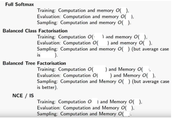
Regularization
-
Define Regularization both intuitively and formally:
Regularization can be, loosely, defined as: any modification we make to a learning algorithm that is intended to reduce its generalization error but not its training error.Formally, it is a set of techniques that impose certain restrictions on the hypothesis space (by adding information) in order to solve an ill-posed problem or to prevent overfitting.
-
Define “well-posedness”:
Hadamard defines Well-Posed Problems as having the properties (1) A Solution Exists (2) It is Unique (3) It’s behavior changes continuously with the initial conditions. - Give four aspects of justification for regularization (theoretical):
- From a philosophical pov:
It attempts to impose Occam’s razor on the solution. - From a probabilistic pov:
From a Bayesian point of view, many regularization techniques correspond to imposing certain prior distributions on model parameters. This is equivalent to making a MAP Estimate of the function we are trying to learn:$$\hat{\boldsymbol{\theta}}_{\mathrm{MAP}}=\underset{\boldsymbol{\theta}}{\arg \min }-\left(\sum_{i=1}^{n} \log \left[p\left(y_{i} | \mathbf{x}_ {i}, \boldsymbol{\theta}\right)\right]\right)-\log [p(\boldsymbol{\theta})]$$
- From an SLT pov:
Regularization can be motivated as imposing a restriction on the complexity of a hypothesis space; called, the “capacity”. In SLT, this is called the Approximation-Generalization Tradeoff. Regularization, effectively, works as a way to maneuver that tradeoff by giving preference to certain solutions. This can be described in two ways:- VC-Theory:
The theory results in a very simple, yet informative, inequality that captures the tradeoff, called The Generalization Bound:$$E_{\text {out}}(h) \leq E_{\text {in}}(h)+\Omega(\mathcal{H})$$
But, if we formalize regularization as adding a regularizer (from the MAP estimate above): \(\Omega = \Omega(h)\) a function of the hypothesis \(h\), to the in-sample error \(E_{\text {in}}\), then we get a new “Augmented” Error:
$$E_{\text {aug}}(h) = E_{\text {in}} + \lambda \Omega(h)$$
Notice the correspondence between the form of the new augmented error \(E_{\text {aug}}\) and the VC Inequality:
$$\begin{aligned}E_{\text {aug}}(h) &= E_{\text {in}}(h) + \lambda \Omega(h) \\ &\downarrow \\ E_{\text {out}}(h) &\leq E_{\text {in}}(h)+\Omega(\mathcal{H})\end{aligned}$$
(we can relate the complexity of a single object to the complexity of a set of objects)
Interpreting the correspondence:
Consider the goal of ML: “to find an in-sample estimate of the out-sample error”. From that perspective, the Augmented Error \(E_{\text {aug}}(h)\) is a better proxy to (estimate of) the out-sample error. Thus, minimizing \(E_{\text {aug}}(h)\) corresponds, better, to minimizing \(E_{\text {out}}(h)\). Where \(\Omega(h)\) is an estimate of \(\Omega(\mathcal{H})\); the regularization term a minimizer of the complexity term. - Bias-Variance Decomposition:
If the variance term \(\operatorname{Var}[h]\) corresponds to the complexity term \(\Omega(\mathcal{H})\), and the regularization term \(\Omega(h)\), also, corresponds to \(\Omega(\mathcal{H})\); then, the regularization term must also correspond to the variance term.
From that perspective, adding the regularization term to the augmented error accounts for the variance of the hypothesis and acts as a measure for it. Thus, minimizing the regularization term \(\Omega(h)\) corresponds to minimizing the variance \(\operatorname{Var}[h]\). However, when the variance of a model goes down the bias tends to go up. Since this inverse-relationship is not linear, this analysis/view gives us a way to apply regularization effectively, by allowing us to measure the effect of regularization.
Basically, we would like our regularization term to reduce the variance more than it increases the bias. We can control that tradeoff by the hyperparameter \(\lambda\).
- VC-Theory:
-
From a practical pov (relating to the real-world):
Most applications of DL are to domains where the true data-generating process is almost certainly outside the model family (hypothesis space). Deep learning algorithms are typically applied to extremely complicated domains such as images, audio sequences and text, for which the true generation process essentially involves simulating the entire universe.Thus, controlling the complexity of the mdoel is not a simple matter of finding the model of the right size, with the right number of parameters; instead, the best fitting model (wrt. generalization error) is a large model that has been regularized appropriately.
- From a philosophical pov:
- Describe an overview of regularization in DL. How does it usually work?
In the context of DL, most regularization strategies are based on regularizing estimators, which usually works by trading increased bias for reduced variance.- Intuitively, how can a regularizer be effective?
An effective regularizer is one that makes a profitable trade, reducing variance significantly while not overly increasing the bias.
- Intuitively, how can a regularizer be effective?
- Describe the relationship between regularization and capacity:
Regularization is a (more general) way of controlling a models capacity by allowing us to express preference for one function over another in the same hypothesis space; instead of including or excluding members from the hypothesis space completely. - Describe the different approaches to regularization:
- Parameter Norm Penalties: \(L^p\) norms, early stopping
- Data Augmentation: noise robustness/injection, dropout
- Semi-supervised Learning
- Multi-task Learning
- Ensemble Learning: bagging, etc.
- Adversarial Training
- Infinite Priors: parameter tying and sharing
- List 9 regularization techniques:
- \(L^2\) regularization
- \(L^1\) regularization
- Dataset Augmentation
- Noise Injection
- Semi-supervised Learning
- Multi-task Learning
- Early Stopping
- Parameter Tying, Sharing
- Sparse Representations
- Ensemble Methods, Bagging etc. 1* Dropout
- Adversarial Training
- Tangent prop and Manifold Tangent Classifier
- Describe Parameter Norm Penalties (PNPs):
Many regularization approaches are based on limiting the capacity of models by adding a parameter norm penalty \(\Omega(\boldsymbol{\theta})\) to the objective function \(J\). We denote the regularized objective function by \(\tilde{J}\):$$\tilde{J}(\boldsymbol{\theta} ; \boldsymbol{X}, \boldsymbol{y})=J(\boldsymbol{\theta} ; \boldsymbol{X}, \boldsymbol{y})+\alpha \Omega(\boldsymbol{\theta}) \tag{7.1}$$
where \(\alpha \in[0, \infty)\) is a HP that weights the relative contribution of the norml penalty term, \(\Omega\), relative to the standard objective function \(J\).
- Define the regularized objective:
$$\tilde{J}(\boldsymbol{\theta} ; \boldsymbol{X}, \boldsymbol{y})=J(\boldsymbol{\theta} ; \boldsymbol{X}, \boldsymbol{y})+\alpha \Omega(\boldsymbol{\theta}) \tag{7.1}$$
- Describe the parameter \(\alpha\):
\(\alpha \in[0, \infty)\) is a HP that weights the relative contribution of the norm penalty term, \(\Omega\), relative to the standard objective function \(J\). - How does it influence the regularization:
- Effects of \(\alpha\):
- \(\alpha = 0\) results in NO regularization
- Larger values of \(\alpha\) correspond to MORE regularization
- Effects of \(\alpha\):
- What is the effect of minimizing the regularized objective?
The effect of minimizing the regularized objective function is that it will decrease, both, the original objective \(J\) on the training data and some measure of the size of the parameters \(\boldsymbol{\theta}\).
- Define the regularized objective:
- How do we deal with the Bias parameter in PNPs? Explain.
In NN, we usually penalize only the weights of the affine transformation at each layer and we leave the biases unregularized.
Biases typically require less data than the weights to fit accurately. The reason is that each weight specifies how TWO variables interact so fitting the weights well, requires observing both variables in a variety of conditions. However, each bias controls only a single variable, thus, we don’t induce too much variance by leaving the biases unregularized. If anything, regularizing the bias can introduce a significant amount of underfitting. - Describe the tuning of the \(\alpha\) HP in NNs for different hidden layers:
In the context of neural networks, it is sometimes desirable to use a separate penalty with a different \(\alpha\) coefficient for each layer of the network. Because it can be expensive to search for the correct value of multiple hyperparameters, it is still reasonable to use the same weight decay at all layers just to reduce the size of search space. - Formally describe the \(L^2\) parameter regularization:
It is a regularization strategy that drives the weights closer to the origin by adding a regularization term:$$\Omega(\mathbf{\theta}) = \frac{1}{2}\|\boldsymbol{w}\|_ {2}^{2}$$
to the objective function.
- AKA:
In statistics, \(L^2\) regularization is also known as Ridge Regression or Tikhonov Regularization.
In ML, it is known as weight decay. - Describe the regularization contribution to the gradient in a single step.
The addition of the weight decay term has modified the learning rule to multiplicatively shrink the weight vector by a constant factor on each step, just before performing the usual gradient update.$$\boldsymbol{w} \leftarrow(1-\epsilon \alpha) \boldsymbol{w}-\epsilon \nabla_{\boldsymbol{w}} J(\boldsymbol{w} ; \boldsymbol{X}, \boldsymbol{y}) \tag{7.5}$$
- Describe the regularization contribution to the gradient. How does it scale?
The effect of weight decay is to rescale \(\boldsymbol{w}^{\ast}\) along the axes defined by the eigenvector of \(\boldsymbol{H}\). Specifically, the component of \(\boldsymbol{w}^{\ast}\) that is aligned with the \(i\)-th eigenvector of \(\boldsymbol{H}\) is rescaled by a factor of \(\frac{\lambda_{i}}{\lambda_{i}+\alpha}\). -
How does weight decay relate to shrinking the individual weight wrt their size? What is the measure/comparison used?
Only directions along which the parameters contribute significantly to reducing the objective function are preserved relatively intact. In directions that do not contribute to reducing the objective function, a small eigenvalue of the Hessian tells us that movement in this direction will not significantly increase the gradient. Components of the weight vector corresponding to such unimportant directions are decayed away through the use of the regularization throughout training.Condition Effect of Regularization \(\lambda_{i}>>\alpha\) Not much \(\lambda_{i}<<\alpha\) The weight value almost shrunk to \(0\)
- AKA:
- Draw a graph describing the effects of \(L^2\) regularization on the weights:
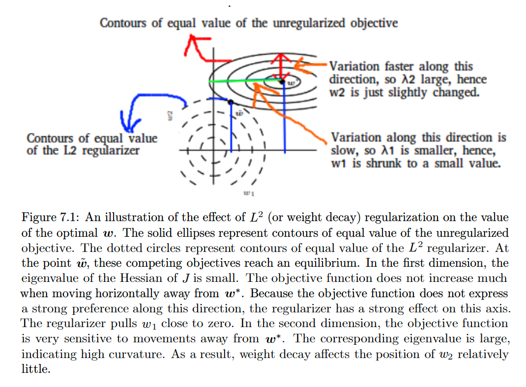
- Describe the effects of applying weight decay to linear regression
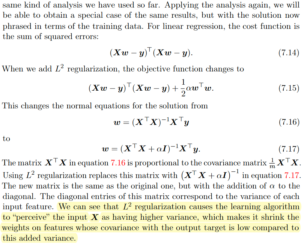
- Derivation:
We place a Gaussian Prior on the weights, with zero mean and equal variance \(\tau^2\):$$\begin{aligned} \hat{\theta}_ {\mathrm{MAP}} &=\arg \max_{\theta} \log P(y | \theta)+\log P(\theta) \\ &=\arg \max _{\boldsymbol{w}}\left[\log \prod_{i=1}^{n} \dfrac{1}{\sigma \sqrt{2 \pi}} e^{-\dfrac{\left(y_{i}-\boldsymbol{w}^T\boldsymbol{x}_i\right)^{2}}{2 \sigma^{2}}}+\log \prod_{j=0}^{p} \dfrac{1}{\tau \sqrt{2 \pi}} e^{-\dfrac{w_{j}^{2}}{2 \tau^{2}}} \right] \\ &=\arg \max _{\boldsymbol{w}} \left[-\sum_{i=1}^{n} \dfrac{\left(y_{i}-\boldsymbol{w}^T\boldsymbol{x}_i\right)^{2}}{2 \sigma^{2}}-\sum_{j=0}^{p} \dfrac{w_{j}^{2}}{2 \tau^{2}}\right] \\ &=\arg \min_{\boldsymbol{w}} \dfrac{1}{2 \sigma^{2}}\left[\sum_{i=1}^{n}\left(y_{i}-\boldsymbol{w}^T\boldsymbol{x}_i\right)^{2}+\dfrac{\sigma^{2}}{\tau^{2}} \sum_{j=0}^{p} w_{j}^{2}\right] \\ &=\arg \min_{\boldsymbol{w}} \left[\sum_{i=1}^{n}\left(y_{i}-\boldsymbol{w}^T\boldsymbol{x}_i\right)^{2}+\lambda \sum_{j=0}^{p} w_{j}^{2}\right] \\ &= \arg \min_{\boldsymbol{w}} \left[ \|XW - \boldsymbol{y}\|^2 + \lambda {\|\boldsymbol{w}\|_ 2}^2\right]\end{aligned}$$
- What is \(L^2\) regularization equivalent to?
\(L^2\) regularization is equivalent to MAP Bayesian inference with a Gaussian prior on the weights. - What are we maximizing?
The MAP Estimate of the data. - Derive the MAP Estimate:
$$\begin{aligned} \hat{\theta}_ {\mathrm{MAP}} &=\arg \max_{\theta} P(\theta | y) \\ &=\arg \max_{\theta} \frac{P(y | \theta) P(\theta)}{P(y)} \\ &=\arg \max_{\theta} P(y | \theta) P(\theta) \\ &=\arg \max_{\theta} \log (P(y | \theta) P(\theta)) \\ &=\arg \max_{\theta} \log P(y | \theta)+\log P(\theta) \end{aligned}$$
- What kind of prior do we place on the weights? What are its parameters?
We place a Gaussian Prior on the weights, with zero mean and equal variance \(\tau^2\).
- What is \(L^2\) regularization equivalent to?
- List the properties of \(L^2\) regularization:
- Notice that L2-regularization has a rotational invariance. This actually makes it more sensitive to irrelevant features.
- Adding L2-regularization to a convex function gives a strongly-convex function. So L2-regularization can make gradient descent converge much faster.
- Formally describe the \(L^1\) parameter regularization:
\(L^1\) Regularization is another way to regulate the model by penalizing the size of its parameters; the technique adds a regularization term:$$\Omega(\boldsymbol{\theta})=\|\boldsymbol{w}\|_{1}=\sum_{i}\left|w_{i}\right| \tag{7.18}$$
which is a sum of absolute values of the individual parameters.
- AKA:
LASSO. - Whats the regularized objective function?
$$\tilde{J}(\boldsymbol{w} ; \boldsymbol{X}, \boldsymbol{y})=\alpha\|\boldsymbol{w}\|_ {1}+J(\boldsymbol{w} ; \boldsymbol{X}, \boldsymbol{y}) \tag{7.19}$$
- What is its gradient?
$$\nabla_{\boldsymbol{w}} \tilde{J}(\boldsymbol{w} ; \boldsymbol{X}, \boldsymbol{y})=\alpha \operatorname{sign}(\boldsymbol{w})+\nabla_{\boldsymbol{w}} J(\boldsymbol{X}, \boldsymbol{y} ; \boldsymbol{w}) \tag{7.20}$$
- Describe the regularization contribution to the gradient compared to L2. How does it scale?
The regularization contribution to the gradient no longer scales linearly with each \(w_i\); instead it is a constant factor with a sign = \(\text{sign}(w_i)\).
- AKA:
- List the properties and applications of \(L^1\) regularization:
- Induces Sparser Solutions
- Solutions may be non-unique
- How is it used as a feature selection mechanism?
LASSO: The Least Absolute Shrinkage and Selection Operator integrates an \(L^1\) penalty with a linear model and a least-squares cost function.
The \(L^1\) penalty causes a subset of the weights to become zero, suggesting that the corresponding features may safely be discarded.
- Derivation:
$$\begin{aligned} \hat{\theta}_ {\mathrm{MAP}} &=\arg \max_{\theta} \log P(y | \theta)+\log P(\theta) \\ &=\arg \max _{\boldsymbol{w}}\left[\log \prod_{i=1}^{n} \dfrac{1}{\sigma \sqrt{2 \pi}} e^{-\dfrac{\left(y_{i}-\boldsymbol{w}^T\boldsymbol{x}_i\right)^{2}}{2 \sigma^{2}}}+\log \prod_{j=0}^{p} \dfrac{1}{2 b} e^{-\dfrac{\left|\theta_{j}\right|}{2 b}} \right] \\ &=\arg \max _{\boldsymbol{w}} \left[-\sum_{i=1}^{n} \dfrac{\left(y_{i}-\boldsymbol{w}^T\boldsymbol{x}_i\right)^{2}}{2 \sigma^{2}}-\sum_{j=0}^{p} \dfrac{\left|w_{j}\right|}{2 b}\right] \\ &=\arg \min_{\boldsymbol{w}} \dfrac{1}{2 \sigma^{2}}\left[\sum_{i=1}^{n}\left(y_{i}-\boldsymbol{w}^T\boldsymbol{x}_i\right)^{2}+\dfrac{\sigma^{2}}{b} \sum_{j=0}^{p}\left|w_{j}\right|\right] \\ &=\arg \min_{\boldsymbol{w}} \left[\sum_{i=1}^{n}\left(y_{i}-\boldsymbol{w}^T\boldsymbol{x}_i\right)^{2}+\lambda \sum_{j=0}^{p}\left|w_{j}\right|\right] \\ &= \arg \min_{\boldsymbol{w}} \left[ \|XW - \boldsymbol{y}\|^2 + \lambda \|\boldsymbol{w}\|_ 1\right]\end{aligned}$$
- What is \(L^1\) regularization equivalent to?
MAP Bayesian inference with an isotropic Laplace distribution prior on the weights. - What kind of prior do we place on the weights? What are its parameters?
Isotropic Laplace distribution prior on the weights: \(\operatorname{Laplace}\left(w_{i} ; 0, \frac{1}{\alpha}\right)\).
- What is \(L^1\) regularization equivalent to?
-
Analyze \(L^1\) vs \(L^2\) regularization:
They both shrink the weights towards zero.\(L^2\) \(L^1\) Sensitive to irrelevant features Robust to irrelevant features Computationally Efficient Non-Differentiable at \(0\) No Sparse Solutions Produces Sparse Solutions No Feature Selection Built-in Feature Selection Unique Solution Possibly multiple solutions - For Sparsity:
The analysis above shows that \(L^1\) produces sparse solutions by killing certain coefficients/weights. While \(L^2\) does not have this property. - For correlated features:
- Identical features:
- \(L^1\) regularization spreads weight arbitrarily (all weights same sign)
- \(L^2\) regularization spreads weight evenly
- Linearly related features:
- \(L^1\) regularization chooses variable with larger scale, \(0\) weight to others
- \(L^2\) prefers variables with larger scale — spreads weight proportional to scale
- Identical features:
- For optimization:
Adding \(L^2\) regularization to a convex function gives a strongly-convex function. So L2-regularization can make gradient descent converge much faster. Moreover, it has analytic solutions and is differentiable everywhere, making it more computationally efficient. \(L^1\) being Non-Differentiable makes it harder to optimize with gradient-based methods and requires approximations. - Give an example that shows the difference wrt sparsity:
Let’s imagine we are estimating two coefficients in a regression. In \(L^2\) regularization, the solution \(\boldsymbol{w} =(0,1)\) has the same weight as \(\boldsymbol{w}=(\frac{1}{\sqrt{2}}, \frac{1}{\sqrt{2}})\) so they are both treated equally. In \(L^1\) regularization, the same two solutions favor the sparse one:$$\|(1,0)\|_{1}=1<\left\|\left(\frac{1}{\sqrt{2}}, \frac{1}{\sqrt{2}}\right)\right\|_{1}=\sqrt{2}$$
So \(L^2\) regularization doesn’t have any specific built in mechanisms to favor zeroed out coefficients, while \(L^1\) regularization actually favors these sparser solutions.
- For sensitivity:
The rotational invariance of the \(L^2\) regularizer makes it more sensitive to irrelevant features.
- For Sparsity:
- Describe Elastic Net Regularization. Why was it devised? Any properties?
$$\Omega = \lambda\left(\alpha\|w\|_{1}+(1-\alpha)\|w\|_{2}^{2}\right), \alpha \in[0,1]$$
- Combines both \(L^1\) and \(L^2\)
- Used to produce sparse solutions, but to avoid the problem of \(L^1\) solutions being sometimes Non-Unique
- The problem mainly arises with correlated features
- Elastic net regularization tends to have a grouping effect, where correlated input features are assigned equal weights.
- Motivate Regularization for ill-posed problems:
- What is the property that needs attention?
Under-Constrained Problems. Under-determined systems. Specifically, when \(X^TX\) is singular. - What would the regularized solution correspond to in this case?
Many forms of regularization correspond to solving inverting \(\boldsymbol{X}^{\top} \boldsymbol{X}+\alpha \boldsymbol{I}\) instead. - Are there any guarantees for the solution to be well-posed? How/Why?
This regularized matrix, \(\boldsymbol{X}^{\top} \boldsymbol{X}+\alpha \boldsymbol{I}\), is guaranteed to be invertible.
- What is the Linear Algebraic property that needs attention?
\(X^{\top}X\) being singular. - What models are affected by this?
Many linear models (e.g. Linear Regression, PCA) depend on inverting \(\boldsymbol{X}^{\top}\boldsymbol{X}\). - What would the sol correspond to in terms of inverting \(X^{\top}X\):
Many forms of regularization correspond to solving inverting \(\boldsymbol{X}^{\top} \boldsymbol{X}+\alpha \boldsymbol{I}\) instead. - When would \(X^{\top}X\) be singular?
- The data-generating function truly has no variance in some direction.
- No Variance is observed in some direction because there are fewer examples (rows of \(\boldsymbol{X}\)) than input features (columns).
- Describe the Linear Algebraic Perspective. What does it correspond to? [LAP]
Given that the Moore-Penrose pseudoinverse \(\boldsymbol{X}^{+}\) of a matrix \(\boldsymbol{X}\) can solve underdetermined linear equations:$$\boldsymbol{X}^{+}=\lim_{\alpha \searrow 0}\left(\boldsymbol{X}^{\top} \boldsymbol{X}+\alpha \boldsymbol{I}\right)^{-1} \boldsymbol{X}^{\top} \tag{7.29}$$
The equation corresponds to performing linear regression with weight-decay.
- Can models with no closed-form solution be underdetermined? Explain. [CFS]
Models with no closed-form solution can, also, be underdetermined:
Take logistic regression on a linearly separable dataset, if a weight vector \(\boldsymbol{w}\) is able to achieve perfect classification, then so does \(2\boldsymbol{w}\) but with even higher likelihood. Thus, an iterative optimization procedure (sgd) will continually increase the magnitude of \(\boldsymbol{w}\) and, in theory, will never halt. - What models are affected by this? [CFS]
Many models that use MLE, log-likelihood/cross-entropy. Namely, Logistic Regression.
- Define the Moore-Penrose Pseudoinverse:
$$\boldsymbol{X}^{+}=\lim_{\alpha \searrow 0}\left(\boldsymbol{X}^{\top} \boldsymbol{X}+\alpha \boldsymbol{I}\right)^{-1} \boldsymbol{X}^{\top} \tag{7.29}$$
- What can it solve? How?
It can solve underdetermined linear equations.
When applied to underdetermined systems w/ non-unique solutions; It finds the minimum norm solution to a linear system. - What does it correspond to in terms of regularization?
The equation corresponds to performing linear regression with weight-decay. - What is the limit wrt?
\(7.29\) is the limit of eq \(7.17\) as the regularization coefficient \(\alpha\) shrinks to zero. - How can we interpret the pseudoinverse wrt regularization?
We can thus interpret the pseudoinverse as stabilizing underdetermined problems using regularization.
- Explain the problem with Logistic Regression:
Logistic regression on a linearly separable dataset, if a weight vector \(\boldsymbol{w}\) is able to achieve perfect classification, then so does \(2\boldsymbol{w}\) but with even higher likelihood. Thus, an iterative optimization procedure (sgd) will continually increase the magnitude of \(\boldsymbol{w}\) and, in theory, will never halt. - What are the possible solutions?
Regularization: e.g. weight decay. - Are there any guarantees that we achieve with regularization? How?
We can use regularization to guarantee the convergence of iterative methods applied to underdetermined problems.
Weight decay will cause gradient descent to quit increasing the magnitude of the weights when the slope of the likelihood is equal to the weight decay coefficient.
- What is the property that needs attention?
- Describe dataset augmentation and its techniques:
Having more data is the most desirable thing to improving a machine learning model’s performance. In many cases, it is relatively easy to artificially generate data. - When is dataset augmentation applicable?
For certain problems like classification this approach is readily usable. E.g. for a classification task, we require the model to be invariant to certain types of transformations, of which we can generate data by applying them on our current dataset. - When is it not?
This approach is not applicable to many problems, especially those that require us to learn the true data-distribution first E.g. Density Estimation. - Motivate the Noise Robustness property:
Noise Robustness is an important property for ML models:- For many classification and (some) regression tasks: the task should be possible to solve even if small random noise is added to the input (Local Constancy)
- Moreover, NNs prove not to be very robust to noise.
- How can Noise Robustness motivate a regularization technique?
To increase noise robustness, we will need to somehow teach our models to ignore noise. That can be done by teaching it to model data that is, perhaps, more noisy than what we actually have; thus, regularizing it from purely and completely fitting the training data. -
How can we enhance noise robustness in NN?
By Noise Injection in different parts of the network.- Give a motivation for Noise Injection:
It can be seen as a form of data augmentation. - Where can noise be injected?
- Input Layer
- Hidden Layer
- Weight Matrices
- Output Layer
- Give Motivation, Interpretation and Applications of injecting noise in the different components (from above):
Injecting Noise in the Input Layer:- Motivation:
We have motivated the injection of noise, to the inputs, as a dataset augmentation strategy. - Interpretation:
For some models, the addition of noise with infinitesimal variance at the input of the model is equivalent to imposing a penalty on the norm of the weights (Bishop, 1995a,b).
Injecting Noise in the Hidden Layers:
- Motivation:
We can motivate it as a variation of data augmentation. - Interpretation:
It can be seen as doing data-augmentation at multiple levels of abstraction. - Applications:
The most successful application of this type of noise injection is Dropout.
It can be seen as a process of constructing new inputs by multiplying by noise.
Injecting Noise in the Weight Matrices:
- Interpretation:
- It can be interpreted as a stochastic implementation of Bayesian inference over the weights.
- The Bayesian View:
The Bayesian treatment of learning would consider the model weights to be uncertain and representable via a probability distribution that reflects this uncertainty. Adding noise to the weights is a practical, stochastic way to reflect this uncertainty.
- The Bayesian View:
- It can, also, be interpreted as equivalent a more traditional form of regularization, encouraging stability of the function to be learned.
-
- It can be interpreted as a stochastic implementation of Bayesian inference over the weights.
- Applications:
This technique has been used primarily in the context of recurrent neural networks (Jim et al., 1996; Graves, 2011).
Injecting Noise in the Output Layer:
- Motivation:
- Most datasets have some number of mistakes in the \(y\) labels. It can be harmful to maximize \(\log p(y | \boldsymbol{x})\) when \(y\) is a mistake. One way to prevent this is to explicitly model the noise on the labels.
One can assume that for some small constant \(\epsilon\), the training set label \(y\) is correct with probability \(1-\epsilon\).
This assumption is easy to incorporate into the cost function analytically, rather than by explicitly drawing noise samples (e.g. label smoothing). - MLE with a softmax classifier and hard targets may never converge - the softmax can never predict a probability of exactly \(0\) or \(1\), so it will continue to learn larger and larger weights, making more extreme predictions forever.{: #bodyContents33mle}
- Most datasets have some number of mistakes in the \(y\) labels. It can be harmful to maximize \(\log p(y | \boldsymbol{x})\) when \(y\) is a mistake. One way to prevent this is to explicitly model the noise on the labels.
- Interpretation:
For some models, the addition of noise with infinitesimal variance at the input of the - Applications:
Label Smoothing regularizes a model based on a softmax with \(k\) output values by replacing the hard \(0\) and \(1\) classification targets with targets of \(\dfrac{\epsilon}{k-1}\) and \(1-\epsilon\), respectively.- Applied to MLE problem: Label smoothing, compared to weight-decay, has the advantage of preventing the pursuit of hard probabilities without discouraging correct classification.
- Application in modern NN: (Szegedy et al. 2015)
- Motivation:
- Give an interpretation for injecting noise in the Input layer:
For some models, the addition of noise with infinitesimal variance at the input of the model is equivalent to imposing a penalty on the norm of the weights (Bishop, 1995a,b). - Give an interpretation for injecting noise in the Hidden layers:
It can be seen as doing data-augmentation at multiple levels of abstraction. - What is the most successful application of this technique:
The most successful application of this type of noise injection is Dropout. - Describe the Bayesian View of learning:
The Bayesian treatment of learning would consider the model weights to be uncertain and representable via a probability distribution that reflects this uncertainty. Adding noise to the weights is a practical, stochastic way to reflect this uncertainty. - How does it motivate injecting noise in the weight matrices?
It can be interpreted as a stochastic implementation of Bayesian inference over the weights. - Describe a different, more traditional, interpretation of injecting noise to matrices. What are its effects on the function to be learned?
It can, also, be interpreted as equivalent a more traditional form of regularization, encouraging stability of the function to be learned. - Whats the biggest application for this kind of regularization?
This technique has been used primarily in the context of recurrent neural networks (Jim et al., 1996; Graves, 2011). - Motivate injecting noise in the Output layer:
- Most datasets have some number of mistakes in the \(y\) labels. It can be harmful to maximize \(\log p(y | \boldsymbol{x})\) when \(y\) is a mistake. One way to prevent this is to explicitly model the noise on the labels.
One can assume that for some small constant \(\epsilon\), the training set label \(y\) is correct with probability \(1-\epsilon\).
This assumption is easy to incorporate into the cost function analytically, rather than by explicitly drawing noise samples (e.g. label smoothing). - MLE with a softmax classifier and hard targets may never converge - the softmax can never predict a probability of exactly \(0\) or \(1\), so it will continue to learn larger and larger weights, making more extreme predictions forever.{: #bodyContents33mle}
- Most datasets have some number of mistakes in the \(y\) labels. It can be harmful to maximize \(\log p(y | \boldsymbol{x})\) when \(y\) is a mistake. One way to prevent this is to explicitly model the noise on the labels.
- What is the biggest application of this technique?
Label Smoothing regularizes a model based on a softmax with \(k\) output values by replacing the hard \(0\) and \(1\) classification targets with targets of \(\dfrac{\epsilon}{k-1}\) and \(1-\epsilon\), respectively. - How does it compare to weight-decay when applied to MLE problems?
Applied to MLE problem: Label smoothing, compared to weight-decay, has the advantage of preventing the pursuit of hard probabilities without discouraging correct classification.
- Give a motivation for Noise Injection:
- Define “Semi-Supervised Learning”:
Semi-Supervised Learning is a class of ML tasks and techniques that makes use of both unlabeled examples from \(P(\mathbf{x})\) and labeled examples from \(P(\mathbf{x}, \mathbf{y})\) to estimate \(P(\mathbf{y} | \mathbf{x})\) or predict \(\mathbf{y}\) from \(\mathbf{x}\).- What does it refer to in the context of DL:
In the context of Deep Learning, Semi-Supervised Learning usually refers to learning a representation \(\boldsymbol{h}=f(\boldsymbol{x})\). - What is its goal?
The goal is to learn a representation such that examples from the same class have similar representations. - Give an example in classical ML:
Using unsupervised learning to build representations: PCA, as a preprocessing step before applying a classifier, is a long-standing variant of this approach.
- What does it refer to in the context of DL:
- Describe an approach to applying semi-supervised learning:
Instead of separating the supervised and unsupervised criteria, we can instead have a generative model of \(P(\mathbf{x})\) (or \(P(\mathbf{x}, \mathbf{y})\)) which shares parameters with a discriminative model \(P(\mathbf{y} \vert \mathbf{x})\).
The idea is to share the unsupervised/generative criterion with the supervised criterion to express a prior belief that the structure of \(P(\mathbf{x})\) (or \(P(\mathbf{x}, \mathbf{y})\)) is connected to the structure of \(P(\mathbf{y} \vert \mathbf{x})\), which is captured by the shared parameters.
By controlling how much of the generative criterion is included in the total criterion, one can find a better trade-off than with a purely generative or a purely discriminative training criterion (Lasserre et al., 2006; Larochelle and Bengio, 2008). -
How can we interpret dropout wrt data augmentation?
Dropout can be seen as a process of constructing new inputs by multiplying by noise. - Describe Multitask Learning as regularization:
The idea is to improve the generalization error by pooling together examples from multiple tasks. Similar to how more data leads to more generalization, using a part of the model for different tasks constrains that part to learn good values. - List the types:
- Add Answers from link below for L2 applied to linear regression and how it reduces variance:
Link -
When is Ridge regression favorable over Lasso regression? for correlated features?
If there exists a subset consisting of few variables that have medium / large sized effect, use lasso regression. In presence of many variables with small / medium sized effect, use ridge regression.?? (ESL authors)If features are correlated, it is so hard to determine which variables to drop, it is often better not to drop variables. Thus, use ridge over lasso since the latter produces non-unique solutions and might drop random features; while former, spreads weight more evenly.
Misc.
- Explain Latent Dirichlet Allocation (LDA)
Latent Dirichlet Allocation (LDA) is a common method of topic modeling, or classifying documents by subject matter.
LDA is a generative model that represents documents as a mixture of topics that each have their own probability distribution of possible words.
The “Dirichlet” distribution is simply a distribution of distributions. In LDA, documents are distributions of topics that are distributions of words. - How to deal with curse of dimensionality
- Feature Selection
- Feature Extraction
- How to detect correlation of “categorical variables”?
- Chi-Squared test
- Define “marginal likelihood” (wrt naive bayes):
Marginal likelihood is, the probability that the word ‘FREE’ is used in any message (not given any other condition?). - KNN VS K-Means
- KNN: Supervised, Classification/Regression Algorithm
- K-Means: Unsupervised Clustering Algorithm
-
When is Ridge regression favorable over Lasso regression for correlated features?
If there are exists a subset consisting of few variables that have medium / large sized effect, use lasso regression. In presence of many variables with small / medium sized effect, use ridge regression.?? (ESL authors)If features are correlated; it is so hard to determine which variables to drop, it is often better not to drop variables. Thus, use ridge over lasso since the latter produces non-unique solutions and might drop random features; while former, spreads weight more evenly.
- What is convex hull ?
In case of linearly separable data, convex hull represents the outer boundaries of the two group of data points. Once convex hull is created, we get maximum margin hyperplane (MMH) as a perpendicular bisector between two convex hulls. MMH is the line which attempts to create greatest separation between two groups. - Do you suggest that treating a categorical variable as continuous variable would result in a better predictive model?
For better predictions, categorical variable can be considered as a continuous variable only when the variable is ordinal in nature. - OLS vs MLE
They both estimate parameters in the model. They are the same in the case of normal distribution. - What are collinearity and multicollinearity?
- Collinearity occurs when two predictor variables (e.g., x1 and x2) in a multiple regression have some correlation.
- Multicollinearity occurs when more than two predictor variables (e.g., x1, x2, and x3) are inter-correlated.
- Describe ways to overcome scaling (scalability) issues:
nystrom methods/low-rank kernel matrix approximations, random features, local by query/near neighbors- Topic Modeling vs Document Classification:
- Text Classification is a form of supervised learning, hence the set of possible classes are known/defined in advance, and won’t change.
- Topic Modeling is a form of unsupervised learning (akin to clustering), so the set of possible topics are unknown apriori. They’re defined as part of generating the topic models.
- Topic Modeling vs Document Classification:
- Why are deep networks better than shallow ones?
Both shallow and deep networks are capable of approximating any function. For the same level of accuracy, deeper networks can be much more efficient in terms of computation and number of parameters. Deeper networks are able to create deep representations, at every layer, the network learns a new, more abstract representation of the input. - What is backpropagation?
Backpropagation is a training algorithm used for a multilayer neural networks. It moves the error information from the end of the network to all the weights inside the network and thus allows for efficient computation of the gradient.
Neural Network Simulator
The backpropagation algorithm can be divided into several steps:- Forward propagation of training data through the network in order to generate output.
- Use target value and output value to compute error derivative with respect to output activations.
- Backpropagate to compute the derivative of the error with respect to output activations in the previous layer and continue for all hidden layers.
- Use the previously calculated derivatives for output and all hidden layers to calculate the error derivative with respect to weights.
- Update the weights.
-
How do you avoid Overfitting?
- How do you avoid Underfitting?
- What is the difference between covariance and correlation?
Correlation is the standardized form of covariance.
Covariances are difficult to compare. For example: if we calculate the covariances of salary ($) and age (years), we’ll get different covariances which can’t be compared because of having unequal scales. To combat such situation, we calculate correlation to get a value between -1 and 1, irrespective of their respective scale.
FeedForward Neural Network
- Define “FeedForward Neural Network”:
The FeedForward Neural Network (FNN) is an artificial neural network wherein the connections between the nodes do not form a cycle, allowing the information to move only in one direction, forward, from the input layer to the subsequent layers. - What is the Architecture of an FFN:
An FNN consists of one or more layers, each consisting of nodes (simulating biological neurons) that hold a certain wight value \(w _ {ij}\). Those weights are usually multiplied by the input values (in the input layer) in each node and, then, summed; finally, one can apply some sort of activation function on the multiplied values to simulate a response (e.g. 1-0 classification). - List the Classes of FNNs:
There are many variations of FNNs. As long as they utilize FeedForward control signals and have a layered structure (described above) they are a type of FNN:- Single-Layer Perceptron
- Multi-Layer Perceptron
- Describe the “Single-Layer Perceptron”:
A linear binary classifier, the single-layer perceptron is the simplest feedforward neural network.
It consists of a single layer of output nodes; the inputs are multiplied by a series of weights, effectively, being fed directly to the outputs where they values are summed in each node, and if the value is above some threshold (typically 0) the neuron fires and takes the activated value (typically 1); otherwise it takes the deactivated value (typically 0).$$f(\mathbf{x})=\left\{\begin{array}{ll}{1} & {\text { if } \mathbf{w} \cdot \mathbf{x}+b>0} \\ {0} & {\text { otherwise }}\end{array}\right.$$
In the context of neural networks, a perceptron is an artificial neuron using the Heaviside step function as the activation function.
- Describe the “Multi-Layer Perceptron”:
This class of networks consists of multiple layers of computational units, usually interconnected in a feed-forward way. Each neuron in one layer has directed connections to the neurons of the subsequent layer.
In many applications the units of these networks apply a sigmoid function as an activation function.
Multilayer Perceptron
- Define the “Multi-Layer Perceptron”:
The Multilayer Perceptron (MLP) is a class of FeedForward Neural Networks that is used for learning from data. - What is the Architecture of an MLP:
- What are the Layers:
The MLP consists of at least three layers of nodes: input layer, hidden layer, and an output layer. - What are the Connections:
The layers in a neural network are connected by certain weights and the MLP is known as a fully-connected network where each neuron in one layer is connected with a weight \(w_{ij}\) to every node in the following layer. - What else is important to make it multi-layer? why?
Each node (except for the input nodes) uses a non-linear activation function that were developed to model the frequency of action potential (firing) of biological neurons.
- What are the Layers:
- Describe “Learning” of an MLP:
The MLP employs a supervised learning technique called backpropagation.
Learning occurs by changing the weights, connecting the layers, based on the amount of error in the output compared to the expected result. Those weights are changed by using gradient-methods to optimize a, given, objective function (called the loss function). - List the properties of the MLP:
- Due to their non-linearity, MLPs can distinguish and model non-linearly-separable data
- According to Cybenko’s Theorem, MLPs are universal function approximators; thus, they can be used for regression analysis and, by extension, classification
- Without the non-linear activation functions, MLPs will be identical to Perceptrons, since Linear Algebra shows that the linear transformations in many hidden layers can be collapsed into one linear-transformation
Deep Feedforward Neural Networks
- Describe the Deep Feedforward Neural Networks:
- As a “Classifier”:
Given \(y=f^{\ast}(\boldsymbol{x})\), a DNN maps an input \(\boldsymbol{x}\) to a category \(y\). - How does it solve the Classification/Regression Problems?
An FNN defines a mapping \(\boldsymbol{y}=f(\boldsymbol{x} ; \boldsymbol{\theta})\) and learns the value of the parameters \(\boldsymbol{\theta}\) that result in the best function approximation. - How does it model the targets?
It models the targets \(\boldsymbol{y}\) as a function \(\boldsymbol{y}=f(\boldsymbol{x} ; \boldsymbol{\theta})\). - What does it learn?
It learns parameters \(\boldsymbol{\theta}\) that result would best approximate the data. - What is its goal?
A balance between:- Function Approximation
- Statistical Generalization
- Why are they called “networks”/how are they represented?:
- FNNs are called networks because they are typically represented by composing together many different functions.
- The model is associated with a DAG describing how the functions are composed together.
- Functions connected in a chain structure are the most commonly used structure of neural networks.
E.g. we might have three functions \(f^{(1)}, f^{(2)},\) and \(f^{(3)}\) connected in a chain, to form \(f(\boldsymbol{x})=f^{(3)}\left(f^{(2)}\left(f^{(1)}(\boldsymbol{x})\right)\right)\); being called the \(n\)-th Layer respectively.
- How are the Functions composed together?
Functions connected in a chain structure are the most commonly used structure of neural networks.
E.g. we might have three functions \(f^{(1)}, f^{(2)},\) and \(f^{(3)}\) connected in a chain, to form \(f(\boldsymbol{x})=f^{(3)}\left(f^{(2)}\left(f^{(1)}(\boldsymbol{x})\right)\right)\); being called the \(n\)-th Layer respectively. - How is this composition described?
The model is associated with a DAG describing how the functions are composed together. - How do we define Depth:
The overall length of the chain is the depth of the model. - What does the Training Data provide? and how do we learn from it?
During training, we drive \(f(\boldsymbol{x})\) to match \(f^{\ast}(\boldsymbol{x}) = \boldsymbol{y}\).
The training data provides us with noisy, approximate examples of \(f^{\ast}(\boldsymbol{x})\) evaluated at different training points.
- As a “Classifier”:
- Describe the Motivation for Deep FFNs:
We can motivate Deep FFNs as an extension of linear models.
The biggest limitation of linear models is that model capacity is limited to linear functions.
To extend linear models to represent non-linear functions of \(\boldsymbol{x}\) we can:- Apply the linear model not to \(\boldsymbol{x}\) itself but to a transformed input \(\phi(\boldsymbol{x})\), where \(\phi\) is a nonlinear transformation.
- Equivalently, apply the kernel trick to obtain nonlinear learning algorithm based on implicitly applying the \(\phi\) mapping.
We can think of \(\phi\) as providing a set of features describing \(\boldsymbol{x}\), or as providing a new representation for \(\boldsymbol{x}\).
Choosing the mapping \(\phi\):
- Use a very generic \(\phi\), s.a. infinite-dimensional (RBF) kernel.
Problems:- If \(\phi(\boldsymbol{x})\) is of high enough dimension, we can always have enough capacity to fit the training set, but generalization to the test set often remains poor.
- Very generic feature mappings are usually based only on the principle of local smoothness and do not encode enough prior information to solve advanced problems.
- Manually Engineer \(\phi\).
Problems:- Requires decades of human effort and the results are usually poor and non-scalable.
- The strategy of deep learning is to learn \(\phi\). We have a model:
- We have a model:
$$y=f(\boldsymbol{x} ; \boldsymbol{\theta}, \boldsymbol{w})=\phi(\boldsymbol{x} ; \boldsymbol{\theta})^{\top} \boldsymbol{w}$$
We now have parameters \(\theta\) that we use to learn \(\phi\) from a broad class of functions, and parameters \(\boldsymbol{w}\) that map from \(\phi(\boldsymbol{x})\) to the desired output.
This is an example of a deep FNN, with \(\phi\) defining a hidden layer. - This approach is the only one of the three that gives up on the convexity of the training problem, but the benefits outweigh the harms.
- In this approach, we parametrize the representation as \(\phi(\boldsymbol{x}; \theta)\) and use the optimization algorithm to find the \(\theta\) that corresponds to a good representation.
- Advantages:
- Capturing the benefit of the first approach:
by being highly generic — we do so by using a very broad family \(\phi(\boldsymbol{x};\theta)\). - Capturing the benefit of the second approach:
Human practitioners can encode their knowledge to help generalization by designing families \(\phi(\boldsymbol{x}; \theta)\) that they expect will perform well.
The advantage is that the human designer only needs to find the right general function family rather than finding precisely the right function.
- Capturing the benefit of the first approach:
- We have a model:
Thus, we can motivate Deep NNs as a way to do automatic, non-linear feature extraction from the inputs.
- topic:
- Interpretation of Neural Networks
It is best to think of feedforward networks as function approximation machines that are designed to achieve statistical generalization, occasionally drawing some insights from what we know about the brain, rather than as models of brain function.
AutoEncoders
- What is an AutoEncoder? What is its goal? (draw a diagram)
An Autoencoder is an ANN used for unsupervised learning of efficient codings/representations.
It aims to learn a good representation (encoding) for a set of data, typically lower-dimensional.
- What type of NN is the Autoencoder?
A Feedforward NN. - Give Motivation for AutoEncoders:
Autoencoder are a generalization of PCA to non-linear projections.
Auto-Encoders allows us to deal with curved manifolds in the input space by using deep layers, where the code is a non-linear function of the input, and the reconstruction of the data from the code is, also, a non-linear function of the code. - Why Deep AutoEncoders? What do they allow us to do?
They provide a really nice way to do non-linear dimensionality reduction:- They provide flexible mappings both ways
- The learning time is linear (or better) in the number of training examples
- The final encoding model/Encoder is fairly compact and fast
- List the Advantages of Depth in AutoEncoders:
- Computational Efficiency: Depth can exponentially reduce the computational cost of representing some functions
- Statistical Efficiency: Depth can exponentially decrease the amount of training data needed to learn some functions
- Representational Efficiency: Experimentally, deep Autoencoders yield better compression compared to shallow or linear Autoencoders
- List the Applications of AutoEncoders (and historical information):
The applications of auto-encoders have changed overtime.
This is due to the advances in the fields that auto-encoders were applied in, or to the incompetency of the auto-encoders.- Historically:
- Information Retrieval
- Anomaly Detection
- Recently, auto-encoders are applied to:
- Data-Denoising
- Dimensionality Reduction (for data visualization)
- Drug discovery
- Historically:
- Describe the Training of Deep AutoEncoders:
- What are the challenges if any?
Training Deep Autoencoders is very challenging:- It is difficult to optimize deep Autoencoders using backpropagation
- With small initial weights the backpropagated gradient dies
- What are the main methods for training Deep AutoEncoders?
- Just initialize the weights carefully as in Echo-State Nets. (No longer used)
- Use unsupervised layer-by-layer pre-training. (Hinton)
This method involves treating each neighbouring set of two layers as a restricted Boltzmann machine so that the pretraining approximates a good solution, then using a backpropagation technique to fine-tune the results. This model takes the name of deep belief network. - Joint Training (most common)
This method involves training the whole architecture together with a single global reconstruction objective to optimize.
- Which one is the superior method?
A study published in 2015 empirically showed that the joint training method not only learns better data models, but also learned more representative features for classification as compared to the layerwise method.
The success of joint training, however, is mostly attributed (depends heavily) on the regularization strategies adopted in the modern variants of the model.
- How is Joint Training better:
It not only learns better data models, but also learned more representative features for classification as compared to the layerwise method. - Why is Joint Training better:
The success of joint training is mostly attributed (depends heavily) on the regularization strategies adopted in the modern variants of the model.
- What are the challenges if any?
- Describe the Architecture of AutoEncoders:
- An auto-encoder consists of:
- An Encoding Function
- A Decoding Function
- A Distance Function
- We choose the encoder and decoder to be parametric functions (typically neural networks), and to be differentiable with respect to the distance function, so the parameters of the encoding/decoding functions can be optimized to minimize the reconstruction loss, using Stochastic Gradient Descent.
- What is the simplest form of an AE:
The simplest form of an Autoencoder is a feedforward neural network (similar to the multilayer perceptron (MLP)) – having an input layer, an output layer and one or more hidden layers connecting them – but with the output layer having the same number of nodes as the input layer, and with the purpose of reconstructing its own inputs (instead of predicting the target value \({\displaystyle Y}\) given inputs \({\displaystyle X}\)). - What realm of “Learning” is employed for AEs?
Self-Supervised Learning.
- An auto-encoder consists of:
- Mathematical Description of the Structure of AutoEncoders:
The encoder and the decoder in an auto-encoder can be defined as transitions \(\phi\) and \({\displaystyle \psi ,}\) such that:$$ {\displaystyle \phi :{\mathcal {X}}\rightarrow {\mathcal {F}}} \\ {\displaystyle \psi :{\mathcal {F}}\rightarrow {\mathcal {X}}} \\ {\displaystyle \phi ,\psi =\arg \min_{\phi ,\psi }\|X-(\psi \circ \phi )X\|^{2}}$$
where \({\mathcal {X} = \mathbf{R}^d}\) is the input space, and \({\mathcal {F} = \mathbf{R}^p}\) is the latent (feature) space, and \(p < d\).
The encoder takes the input \({\displaystyle \mathbf {x} \in \mathbb {R} ^{d}={\mathcal {X}}}\) and maps it to \({\displaystyle \mathbf {z} \in \mathbb {R} ^{p}={\mathcal {F}}}\):
$${\displaystyle \mathbf {z} =\sigma (\mathbf {Wx} +\mathbf {b} )}$$
- The image \(\mathbf{z}\) is referred to as code, latent variables, or latent representation.
- \({\displaystyle \sigma }\) is an element-wise activation function such as a sigmoid function or a rectified linear unit.
- \({\displaystyle \mathbf {W} }\) is a weight matrix
- \({\displaystyle \mathbf {b} }\) is the bias.
The Decoder maps \({\displaystyle \mathbf {z} }\) to the reconstruction \({\displaystyle \mathbf {x'} }\) of the same shape as \({\displaystyle \mathbf {x} }\):
$${\displaystyle \mathbf {x'} =\sigma '(\mathbf {W'z} +\mathbf {b'} )}$$
where \({\displaystyle \mathbf {\sigma '} ,\mathbf {W'} ,{\text{ and }}\mathbf {b'} }\) for the decoder may differ in general from those of the encoder.
Autoencoders minimize reconstruction errors, such as the L-2 loss:
$${\displaystyle {\mathcal {L}}(\mathbf {x} ,\psi ( \phi (\mathbf {x} ) ) ) = {\mathcal {L}}(\mathbf {x} ,\mathbf {x'} )=\|\mathbf {x} -\mathbf {x'} \|^{2}=\|\mathbf {x} -\sigma '(\mathbf {W'} (\sigma (\mathbf {Wx} +\mathbf {b} ))+\mathbf {b'} )\|^{2}}$$
where \({\displaystyle \mathbf {x} }\) is usually averaged over some input training set.
- How do we define the “Encoder” and “Decoder”?
Transition Maps. - The Encoder maps what to what?
The encoder takes the input \({\displaystyle \mathbf {x} \in \mathbb {R} ^{d}={\mathcal {X}}}\) and maps it to \({\displaystyle \mathbf {z} \in \mathbb {R} ^{p}={\mathcal {F}}}\):$${\displaystyle \mathbf {z} =\sigma (\mathbf {Wx} +\mathbf {b} )}$$
- The Decoder maps what to what?
The Decoder maps \({\displaystyle \mathbf {z} }\) to the reconstruction \({\displaystyle \mathbf {x'} }\) of the same shape as \({\displaystyle \mathbf {x} }\):$${\displaystyle \mathbf {x'} =\sigma '(\mathbf {W'z} +\mathbf {b'} )}$$
where \({\displaystyle \mathbf {\sigma '} ,\mathbf {W'} ,{\text{ and }}\mathbf {b'} }\) for the decoder may differ in general from those of the encoder.
- What is the type of loss?
Autoencoders minimize reconstruction errors, such as the L2 loss:$${\displaystyle {\mathcal {L}}(\mathbf {x} ,\psi ( \phi (\mathbf {x} ) ) ) = {\mathcal {L}}(\mathbf {x} ,\mathbf {x'} )=\|\mathbf {x} -\mathbf {x'} \|^{2}=\|\mathbf {x} -\sigma '(\mathbf {W'} (\sigma (\mathbf {Wx} +\mathbf {b} ))+\mathbf {b'} )\|^{2}}$$
where \({\displaystyle \mathbf {x} }\) is usually averaged over some input training set.
- What are “Transition Functions”?
- Compare AutoEncoders and PCA (wrt what they learn):
- List the different Types of AEs
- Vanilla Auto-Encoder
- Sparse Auto-Encoder
- Denoising Auto-Encoder
- Variational Auto-Encoder (VAE)
- Contractive Auto-Encoder.
- How can we use AEs for Initialization?
After training an auto-encoder, we can use the encoder to compress the input data into it’s latent representation (which we can view as features) and input those to the neural-net (e.g. a classifier) for prediction.
- Describe the Representational Power of AEs:
- The universal approximator theorem guarantees that a feedforward neural network with at least one hidden layer can represent an approximation of any function (within a broad class) to an arbitrary degree of accuracy, provided that it has enough hidden units. This means that an Autoencoder with a single hidden layer is able to represent the identity function along the domain of the data arbitrarily well.
- However, the mapping from input to code is shallow. This means that we are not able to enforce arbitrary constraints, such as that the code should be sparse.
- A deep Autoencoder, with at least one additional hidden layer inside the encoder itself, can approximate any mapping from input to code arbitrarily well, given enough hidden units.
- (wrt Layer Size and Depth):
- Why is Depth Important?
- Describe the progression (stages) of AE Architectures in CV:
- Originally: Linear + nonlinearity (sigmoid).
- Later: Deep, fully-connected.
- Later: ReLU CNN (UpConv).
- List the Types of AEs wrt the Bottleneck/Code-Length:
- Undercomplete:
- Overcomplete:
- Complete:
- What are Undercomplete AutoEncoders?
An Undercomplete Autoencoder is one whose code dimension is less than the input dimension. - What’s the motivation behind Undercomplete AEs?
Learning an undercomplete representation forces the autoencoder to capture the most salient features of the training data. - List the Challenges of Training AEs using the Auto-Encoding Objective (case-by-case):
- If an Autoencoder succeeds in simply learning to set \(\psi(\phi (x)) = x\) everywhere, then it is not especially useful.
Instead, Autoencoders are designed to be unable to learn to copy perfectly. Usually they are restricted in ways that allow them to copy only approximately, and to copy only input that resembles the training data. - In Undercomplete Autoencoders If the encoder and decoder are allowed too much capacity, the Autoencoder can learn to perform the copying task without extracting useful information about the distribution of the data.
Theoretically, one could imagine that an Autoencoder with a one-dimensional code but a very powerful nonlinear encoder could learn to represent each training example \(x^{(i)}\) with the code \(i\). This specific scenario does not occur in practice, but it illustrates clearly that an Autoencoder trained to perform the copying task can fail to learn anything useful about the dataset if the capacity of the Autoencoder is allowed to become too great. - A similar problem occurs in Complete AEs
- As well as in the Overcomplete case, in which the hidden code has dimension greater than the input.
In complete and overcomplete cases, even a linear encoder and linear decoder can learn to copy the input to the output without learning anything useful about the data distribution.
- If an Autoencoder succeeds in simply learning to set \(\psi(\phi (x)) = x\) everywhere, then it is not especially useful.
- What is the Main Method/Approach of addressing the Challenges above (Training AEs)?
Regularized Autoencoders.
-
Define Regularized Autoencoders:
Regularized Autoencoders are a variant of Autoencoders that modifies the loss function with regularization techniques to allow us to train any architecture of AEs successfully.-
What’s the Big-Idea/Main-Point behind R-AEs and AEs in general?
A regularized Autoencoder can be nonlinear and overcomplete but still learn something useful about the data distribution even if the model capacity is great enough to learn a trivial identity function. - What does it allow us to do? How*?
It allows us to train any architecture of Autoencoder successfully, choosing the code dimension and the capacity of the encoder and decoder based on the complexity of distribution to be modeled. - How does it address the Challenges? (Compare)
Rather than limiting the model capacity by keeping the Encoder and Decoder shallow and the Code-Size small, they use a loss function that encourages the model to have other (useful) properties besides the ability to copy its input to it output:
- List if any the restrictions/guidelines for setting the capacity of the R-AEs:
We should choose the code dimension and the capacity of the encoder and decoder based on the complexity of distribution to be modeled. - What other Properties does it encourage to be learned?
- Sparsity of the Representation
- Smallness of the Derivative of the Representation
- Robustness to Noise or to Missing Inputs
- What kind of technique (also type) of AEs can be “non-linear” and still learn useful codes?
Regularized AEs. - What kind of technique-needed for (also type-of) AEs can be “overcomplete” and still learn useful codes?
Regularized AEs. - What kind of technique-needed for (also type-of) AEs can be “nonlinear” AND “overcomplete” and still learn useful codes?
Regularized AEs. - What are the ways to learn useful encodings/representations?
Defining an appropriate Objective and Objective Function.- What types of objectives help learn useful encodings/representations?
(regularized/approximate) Auto-Encoding - Maximizing the Probability of training Data (NLL)
Further Info
- What types of objectives help learn useful encodings/representations?
-
-
Describe the Relationship between Generative Models and AEs:
In addition to the traditional AEs described here, nearly any generative model with latent variables and equipped with an inference procedure (for computing latent representations given input) may be viewed as a particular form of Autoencoder.- What are the components needed for the Generative Model?:
- generative model
- latent variables
- inference procedure (for computing latent representations given input)
- What notable types? List:.
The descendants of the Helmholtz machine (Hinton et al., 1995b), such as:
- Variational Autoencoders
- Generative Stochastic Networks
- Compare Generative Models & AEs in how they learn codings/representations:
These models naturally learn high-capacity, overcomplete encodings of the input and do NOT require regularization for these encodings to be useful.
- Why are their representations “naturally” useful?
Their encodings are naturally useful because the models were trained to approximately maximize the probability of the training data rather than to copy the input to the output.
- What are the components needed for the Generative Model?:
-
List the Different Types of Regularized Autoencoders:
- Sparse Autoencoders
- Denoising Autoencoders
- Regularizing by Penalizing Derivatives
- Contractive Autoencoders
- Predictive Sparse Decomposition
- Define Sparse Autoencoders (w/ equation):
Sparse Autoencoders are simply Autoencoders whose training criterion involves a sparsity penalty \(\Omega(\boldsymbol{h})\) on the code layer \(\boldsymbol{h},\) in addition to the reconstruction error:$${\displaystyle {\mathcal {L}}(\mathbf {x} ,\psi ( \phi (\mathbf {x} ) ) ) + \Omega(\boldsymbol{h})}$$
where typically we have \(\boldsymbol{h}=\phi(\boldsymbol{x})\), the encoder output.
- How can we interpret Sparse AEs? (Hint: 3 interpretations)
- Regularization Interpretation
- Bayesian Interpretation
- Latent-Variable Interpretation
- Give the “Regularization” Interpretation of Sparse AEs:
We can think of the penalty \(\Omega(\boldsymbol{h})\) simply as a regularizer term added to a feedforward network whose primary task is to copy the input to the output (unsupervised learning objective) and possibly also perform some supervised task (with a supervised learning objective) that depends on these sparse features. - Give the “Bayesian” Interpretation of Regularized AEs:
Unlike other regularizers such as weight decay, there is not a straightforward Bayesian interpretation to this regularizer.
Regularized Autoencoders defy such an interpretation because the regularizer depends on the data and is therefore by definition not a prior in the formal sense of the word.
We can still think of these regularization terms as implicitly expressing a preference over functions. - Give the “Latent Variable” Interpretation of Sparse AEs:
Rather than thinking of the sparsity penalty as a regularizer for the copying task, we can think of the entire sparse Autoencoder framework as approximating maximum likelihood training of a generative model that has latent variables.
- What do Sparse AEs approximate?
They approximate Latent Variable Models.
Specifically, Generative Models with Latent Variables Trained with Maximum Likelihood. - How do they (does that) relate to MLE?
They approximate Generative Models with Latent Variables Trained with Maximum Likelihood.
- Give the “Regularization” Interpretation of Sparse AEs:
- Define Denoising Autoencoders:
Denoising Autoencoders (DAEs) is an Autoencoder that receives a corrupted data point as input and is trained to predict the original, uncorrupted data point as its output. - What do they minimize? (canonical loss)
$$L(\boldsymbol{x}, g(f(\tilde{\boldsymbol{x}})))$$
where \(\tilde{\boldsymbol{x}}\) is a copy of \(\boldsymbol{x}\) that has been corrupted by some form of noise.
- What do they learn? How? (compare)
They learn to undo the corruption rather than simply copying their input.
The denoising training forces \(\psi\) and \(\phi\) to implicitly learn the structure of \(p_{\text {data}}(\boldsymbol{x})\). - How do we generate the inputs?
We introduce a Corruption Process \(C(\tilde{\mathbf{x}} \vert \mathbf{x})\) which represents a conditional distribution over corrupted samples \(\tilde{\boldsymbol{x}}\), given a data sample \(\boldsymbol{x}\).
- What does the “Corruption Process” represent/define?
It represents a Conditional Distribution over corrupted samples \(\tilde{\boldsymbol{x}}\), given a data sample \(\boldsymbol{x}\).
- What does the “Corruption Process” represent/define?
- How do we generate the training examples (input-output pair)? (process)
- Sample a training example \(\boldsymbol{x}\) from the training data.
- Sample a corrupted version \(\tilde{\boldsymbol{x}}\) from \(C(\tilde{\mathbf{x}} \vert \mathbf{x}=\boldsymbol{x})\)
- Use \((\boldsymbol{x}, \tilde{\boldsymbol{x}})\) as a training example for estimating the Autoencoder reconstruction distribution \(p_{\text {reconstruct }}(\boldsymbol{x} \vert \tilde{\boldsymbol{x}})=p_{\text {decoder }}(\boldsymbol{x} \vert \boldsymbol{h})\) with \(\boldsymbol{h}\) the output of encoder \(f(\tilde{\boldsymbol{x}})\) and \(p_{\text {decoder}}\) typically defined by a decoder \(g(\boldsymbol{h})\).
- What does the Denoising AE learn specifically? (mathematically)
The DAE learns a Reconstruction Distribution \(p_{\text {reconstruct }}(\boldsymbol{x} \vert \tilde{\boldsymbol{x}})=p_{\text {decoder }}(\boldsymbol{x} \vert \boldsymbol{h})\) with \(\boldsymbol{h}\) the output of encoder \(f(\tilde{\boldsymbol{x}})\) and \(p_{\text {decoder}}\) typically defined by a decoder \(g(\boldsymbol{h})\).
- What do we use as an estimate for the “Reconstruction Distribution”?
We use \((\boldsymbol{x}_ i, \tilde{\boldsymbol{x}}_ i)\) as Training Data for estimating the Autoencoder reconstruction distribution \(p_{\text {reconstruct }}(\boldsymbol{x} \vert \tilde{\boldsymbol{x}})\). - What is the output of the encoder \(f\)?
\(f(\tilde{\boldsymbol{x}}) = \boldsymbol{h}\). - What is the output of the decoder \(g\)?
\(g(\boldsymbol{h})=p_{\text {decoder}}(\boldsymbol{x} \vert \boldsymbol{h})=\boldsymbol{x}\). - What is the “Reconstruction Distribution” equal to?
\(p_{\text {reconstruct}}(\boldsymbol{x} \vert \tilde{\boldsymbol{x}})=p_{\text {decoder}}(\boldsymbol{x} \vert \boldsymbol{h})\).
- What do we use as an estimate for the “Reconstruction Distribution”?
- How do we Train the Denoising AE?
Typically we can simply perform gradient-based approximate minimization (such as minibatch gradient descent) on the negative log-likelihood \(-\log p_{\text {decoder}}(\boldsymbol{x} \vert \boldsymbol{h})\).
So long as the encoder is deterministic, the denoising Autoencoder is a feedforward network and may be trained with exactly the same techniques as any other FFN.- What is the Loss?
Negative Log-Likelihood (NLL): \(-\log p_{\text {decoder}}(\boldsymbol{x} \vert \boldsymbol{h})\). - What is the Optimization Method?
SGD. - What is the Training similar to?
So long as the encoder is deterministic, the DAE is a feedforward network (FFN) and may be trained with exactly the same techniques as any other FFN. - Is the Encoder Deterministic?
Yes.- Would change if it was one or the other?
If it were “stochastic” then it can’t be learned w/ max-likelihood training.
- Would change if it was one or the other?
- What is the Loss?
- How can we view the function of DAEs (wrt learning/training) from a Probabilistic pov?
Given above, we can therefore view the DAE as performing stochastic gradient descent on the following expectation:$$-\mathbb{E}_{\mathbf{x} \sim \hat{p}_{\text {data }}(\mathbf{x})} \mathbb{E}_{\tilde{\mathbf{x}} \sim C(\tilde{\mathbf{x}} \vert \boldsymbol{x})} \log p_{\text {decoder}}(\boldsymbol{x} \vert \boldsymbol{h}=f(\tilde{\boldsymbol{x}}))$$
where \(\hat{p}_ {\text {data}}(\mathrm{x})\) is the training distribution.
- What Expectation is it minimizing? Over what?
$$-\mathbb{E}_{\mathbf{x} \sim \hat{p}_{\text {data }}(\mathbf{x})} \mathbb{E}_{\tilde{\mathbf{x}} \sim C(\tilde{\mathbf{x}} \vert \boldsymbol{x})} \log p_{\text {decoder}}(\boldsymbol{x} \vert \boldsymbol{h}=f(\tilde{\boldsymbol{x}}))$$
where \(\hat{p}_ {\text {data}}(\mathrm{x})\) is the training distribution.
- Can we re-write the Objective/Loss wrt the Empirical Distribution?
$$-\mathbb{E}_{\mathbf{x} \sim \hat{p}_{\text {data }}(\mathbf{x})} \mathbb{E}_{\tilde{\mathbf{x}} \sim C(\tilde{\mathbf{x}} \vert \boldsymbol{x})} \log p_{\text {decoder}}(\boldsymbol{x} \vert \boldsymbol{h}=f(\tilde{\boldsymbol{x}}))$$
where \(\hat{p}_ {\text {data}}(\mathrm{x})\) is the training distribution.
- What Expectation is it minimizing? Over what?
- What other ways exist for learning/training DAEs?
Score Matching. -
How do DAEs and VAEs relate to each other?
DAEs learn to represent a probability distribution.
To use the AE as a generative model to draw samples from this distribution, we need to make the Encoder Stochastic: this is known as the Variational Autoencoder. - Define Contractive Autoencoders
Contractive Autoencoders (CAEs) (Rifai et al., 2011a,b) introduces an explicit regularizer on the code \(\boldsymbol{h}=\phi(\boldsymbol{x}),\) encouraging the derivatives of \(\phi\) to be as small as possible:$$\Omega(\boldsymbol{h})=\lambda\left\|\frac{\partial \phi(\boldsymbol{x})}{\partial \boldsymbol{x}}\right\|_ {F}^{2}$$
The penalty \(\Omega(\boldsymbol{h})\) is the squared Frobenius norm (sum of squared elements) of the Jacobian matrix of partial derivatives associated with the encoder function.
- What is the regularizer/penalty used?
The penalty \(\Omega(\boldsymbol{h})\) is the squared Frobenius norm (sum of squared elements) of the Jacobian matrix of partial derivatives associated with the encoder function. - What does it encourage the system to do?
It encouraging the derivatives of the Encoder \(\phi\) to be as small as possible.
- What is the regularizer/penalty used?
- How is the Contractive AE connected to the DAE:
- In the limit of small Gaussian input noise, the denoising reconstruction error is equivalent to a contractive penalty on the reconstruction function that maps \(\boldsymbol{x}\) to \(\boldsymbol{r}=\psi(\phi(\boldsymbol{x}))\). I.e.:
- Denoising Autoencoders: make the reconstruction function resist small but finite-sized perturbations of the input
- Contractive Autoencoders: make the feature extraction function resist infinitesimal perturbations of the input. - When using the Jacobian-based contractive penalty to pretrain features \(\phi(\boldsymbol{x})\) for use with a classifier, the best classification accuracy usually results from applying the contractive penalty to \(\phi(\boldsymbol{x})\) rather than to \(\psi(\phi(\boldsymbol{x}))\).
- A contractive penalty on \(\phi(\boldsymbol{x})\) also has close connections to score matching.
- In the limit of small Gaussian input noise, the denoising reconstruction error is equivalent to a contractive penalty on the reconstruction function that maps \(\boldsymbol{x}\) to \(\boldsymbol{r}=\psi(\phi(\boldsymbol{x}))\). I.e.:
- Why is the CAE called “Contractive”?
The name contractive arises from the way that the CAE warps space.
Specifically, because the CAE is trained to resist perturbations of its input, it is encouraged to map a neighborhood of input points to a smaller neighborhood of output points. We can think of this as contracting the input neighborhood to a smaller output neighborhood.
- Is it contractive locally or globally or both?
The CAE is contractive only locally-all perturbations of a training point \(\boldsymbol{x}\) are mapped near to \(\phi(\boldsymbol{x})\). Globally, two different points \(\boldsymbol{x}\) and \(\boldsymbol{x}^{\prime}\) may be mapped to \(\phi(\boldsymbol{x})\) and \(\psi\left(\boldsymbol{x}^{\prime}\right)\) points that are farther apart than the original points. - Give the Interpretation of the CAE as a Linear Operator:
We can think of the Jacobian matrix \(J\) at a point \(x\) as approximating the nonlinear encoder \(\phi(x)\) as being a linear operator. This allows us to use the word “contractive” more formally.
In the theory of linear operators, a linear operator is said to be contractive if the norm of \(J x\) remains less than or equal to 1 for all unit-norm \(x\). In other words, \(J\) is contractive if it shrinks the unit sphere.
We can think of the CAE as penalizing the Frobenius norm of the local linear approximation of \(\phi(x)\) at every training point \(x\) in order to encourage each of these local linear operator to become a contraction.
- Is it contractive locally or globally or both?
- List the Issues associated with using a “Contractive Penalty”:
- What is an AutoEncoder? Why do we “Auto-Encode”? (Hint: it’s really a misnomer) Why is “AutoEncoder” a misnomer?
AutoEncoders are FFNs with a narrow, low-dimensional bottleneck layer in the middle that learn are used to learn efficient data codings/representations.
The objective for an AE is to learn to copy its input to its output. However, performing the copying task per se would be meaningless, and this is why usually autoencoders are restricted in ways that force them to reconstruct the input only approximately, prioritizing the most relevant aspects of the data to be copied.
i.e. It’s not really a misnomer since the general objective is in the form of “auto-encoding” however, the main goal is not just to learn to reconstruct the data from the code but to learn useful information about the distribution of the data.
The goal is not perform the copying task, but to perform the copying task for the purpose of __ extracting useful information about the distribution of the data__.
The Goal: capture important information and learn richer representations.. - What’s the Big-Idea/Main-Point behind R-AEs and AEs in general?
A regularized Autoencoder can be nonlinear and overcomplete but still learn something useful about the data distribution even if the model capacity is great enough to learn a trivial identity function.- What do DAEs learn to represent?
They learn to represent a probability distribution. - How do Regularized AEs learn Manifolds?
Regularized Autoencoders learn manifolds by balancing two opposing forces. - How can we Learn Manifolds w/ AEs?
- What do DAEs learn to represent?